Exploring the Solar Rooftop Potential of Wortley Village/Old South in London, Ontario using ArcGIS Pro and LiDAR-derived DSM

Over the weekend in my exploration of ArcGIS Notebooks, I came across this very interesting ArcGIS Pro Lesson by Esri Senior Product Engineer Delphine Khanna. Although it was not related to my initial plan of learning how to use ArcGIS Notebooks, the project happened to use ArcGIS Pro which I had installed a few days ago. I decided to give it a try since I was always intrigued to find out the possibility of households in London switching to use solar power. Installing solar panels have becoming more popular nowadays given the rising concerns of climate change and increasing awareness of using sustainable energy. In the past, people were very reluctant to use solar power due to a number of reasons, to list a few:

1. High capital cost of purchasing the panels, and high cost of hiring professionals to do the installation
2. Existing power supply was cheaper and the maintenance cost was shared across the city (why would people go for a more expensive option while there’s already a cheaper and worry-free alternative?)
3. Lack of advertisement and lack of businesses offering the services and products
4. Product selections were very limited and the solar technology itself was not fully developed
5. Roof isn’t suitable

While other factors may remain challenging to solve, there’s at least one thing that GIS technology can do to help people make an “informed decision”, which is to help them identify the potential of their rooftops to harvest the natural energy of the sun (reason#5). Although having this piece of information may not encourage more people to install solar panels due to other reasons mentioned above, I think it’s still very important to raise the awareness of using solar energy, keeping people informed about the rapidly maturing solar technology (check out Tesla’s new solar roof), and what they can do to reduce carbon emissions.

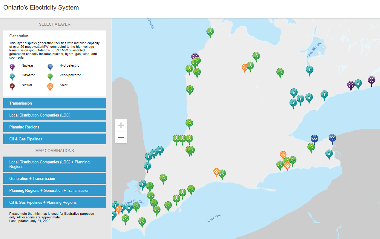
I was able to do a quick search on Ontario’s Eletricity System, and it seems like electricity in London is mainly powered by nearby gas-fired power plants in the GTA and wind farms near Strathroy. However, it’s difficult to determine the primary source of London’s electricity because all power generated from the power plants feed directly into the grid and transmit to the closest stations. It’s interesting to learn that there have been quite a few solar farms being developed in the vicinity of London such as the Silver Creek Solar Farm, the Nanticoke Solar Facility (once the largest coal-powered station), and the Grande Renewable Solar Project (its solar panels are manufactured in London). Statistics from the Canada Energy Regulator also indicates that there have been a growing supply of solar power in recent years, and about “98% of solar capacity in Canada is installed in Ontario, and capable of generating 2871 MW of electricity in 2018“.

So why aren’t more people installing solar roofing or solar panels over their roofs? The answer can be simple: they don’t know if their roofs are suitable and consulting a professional is expensive!

After doing these quick research and learning that solar power is becoming more popular in Ontario, I started exploring the possibility of houses switching to solar power in the Old South Neighbourhood of London, Ontario. A similar community-based study has been conducted in British Columbia by Dr. Rory Tooke using a LiDAR-derived DSM, and I’m hoping to see a similar project to take place in London so more people can contribute to the Climate Action Plan. Here I will share what I learn from Delphine Khanna‘s lesson and what steps I took to complete the project:

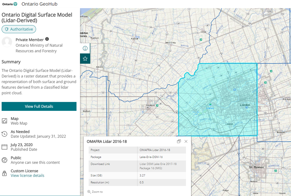
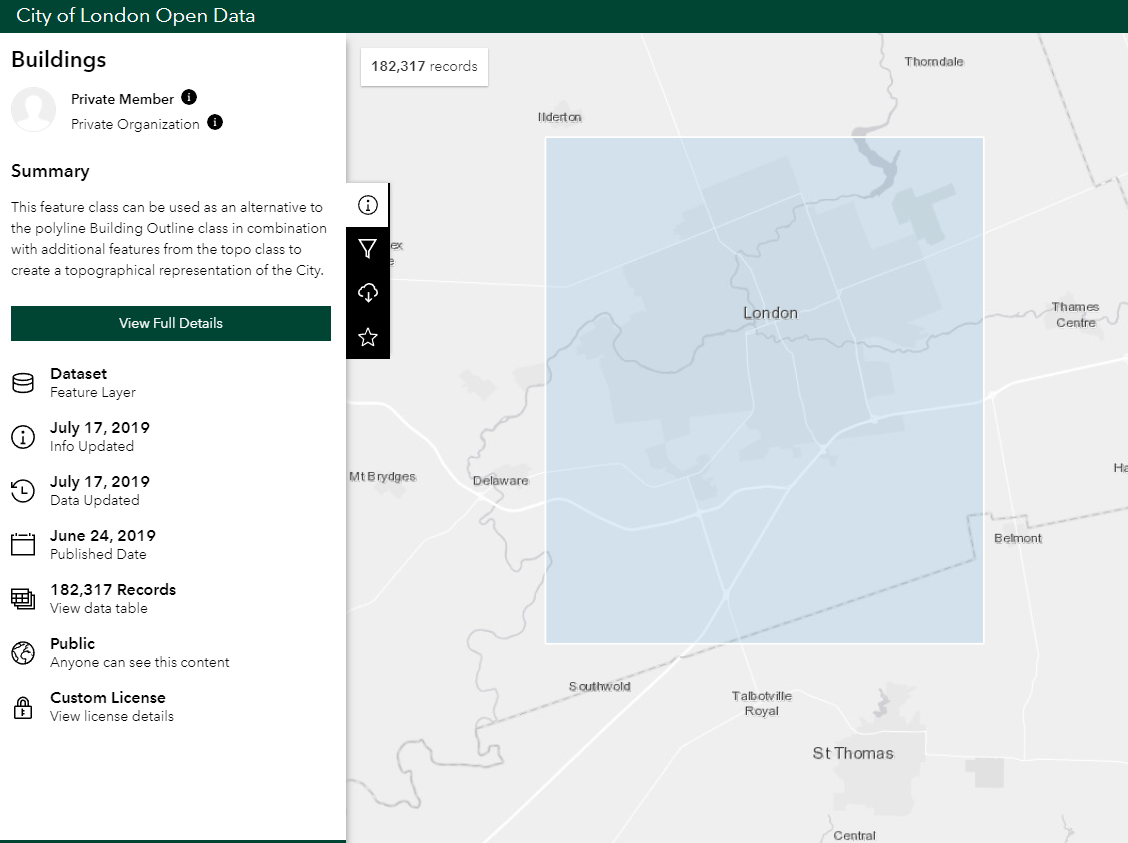
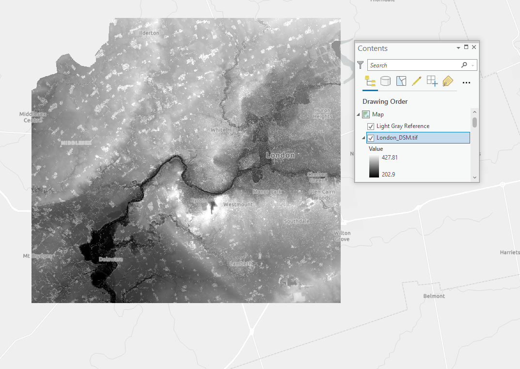
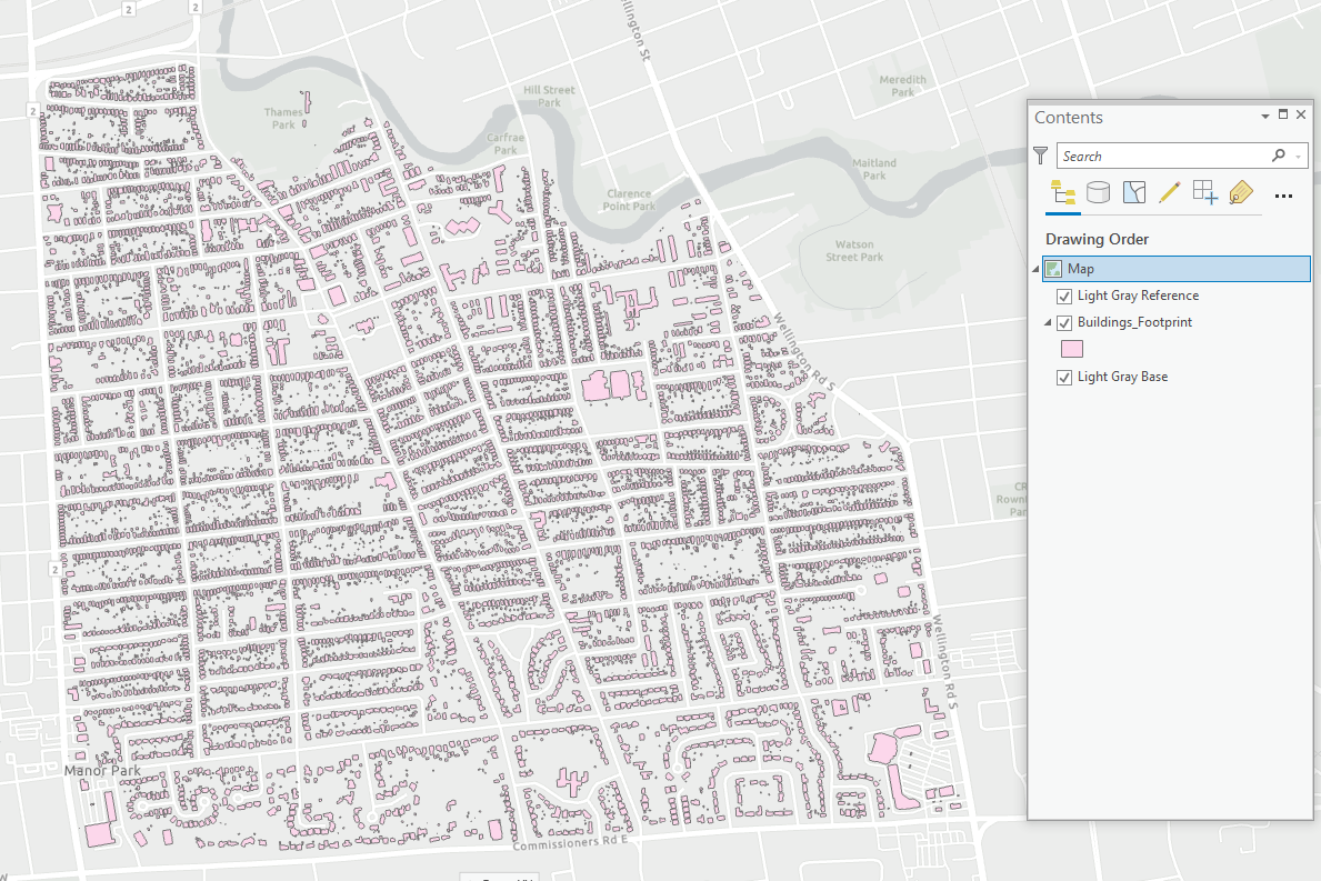
Step 1: Gather the DSM layer and Building Footprints

I was able to download a Lidar-Derived DSM layer from the Ontario GeoHub, and a shapefile that contains all of London’s building footprints from the City of London Open Data portal.

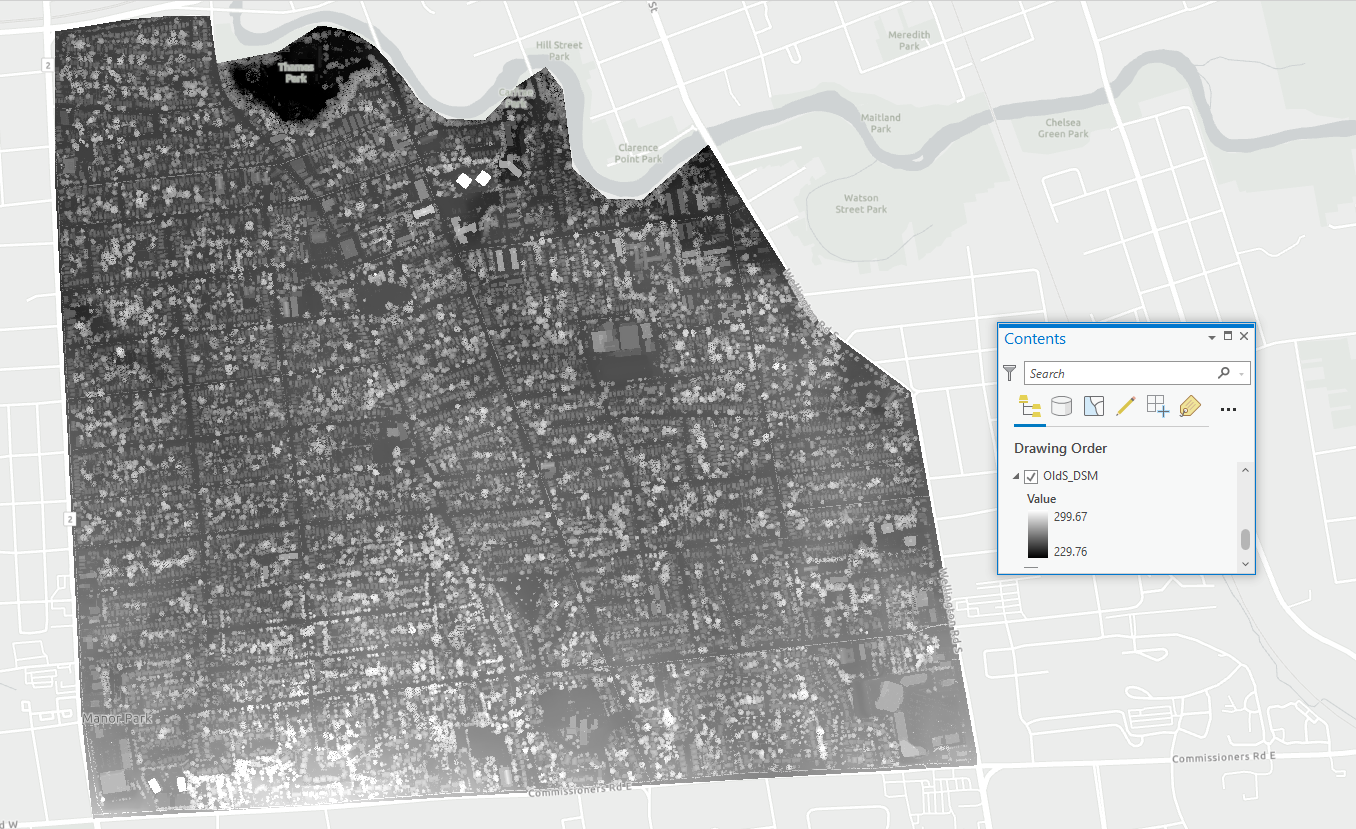
Step 2: Prepping and Extracting the Data for The Study Area

The original datasets from both sites were relatively large. Thus it’s important to select the features only within my chosen study area (Old South Neighbourhood). Usually I’m able to find a map that divides the city into communities or census tracts, but the boundary for Wortley Village/Old South has been unclear thus I decided to manually draw the boundary according to a offical site from City of London.

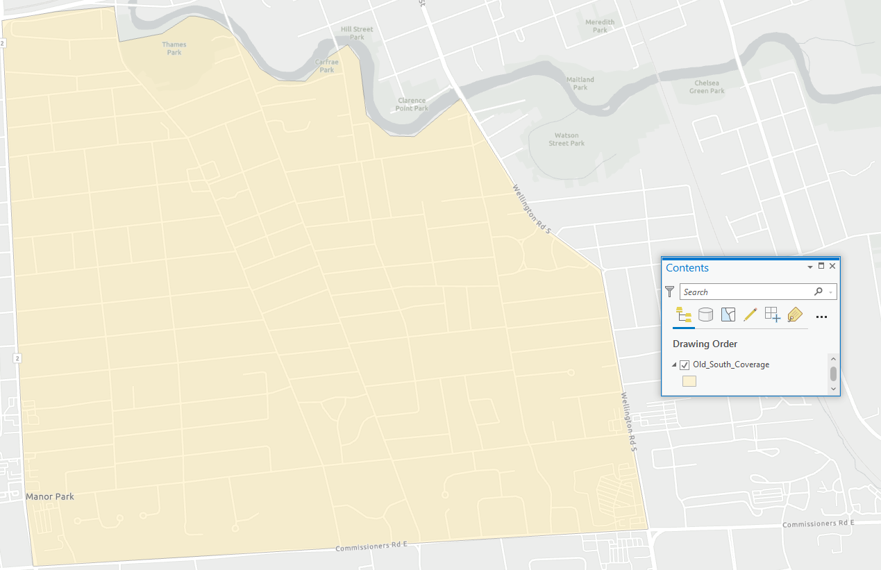
I used this polygon as a “Mask” to extract the data I need from the original datasets. Note that the building footprint dataset is a shapefile so I had to use the “Clip” function, whereas I used the “Extract by Mask” function for the DSM layer because it’s a raster.

The original DSM dataset was composed of hundreds of raster files instead of one large raster file. There was an extra step I needed to do before extracting the data for my study area. I initially attempted using the Combine (Spatial Analyst) tool to stitch all the raster together but it was not successful because there were too many files. I came up with an alternate method by using the Mosaic To New Raster (Data Management) tool to stitch all the rasters together into one single dataset.

Extracted Layers:

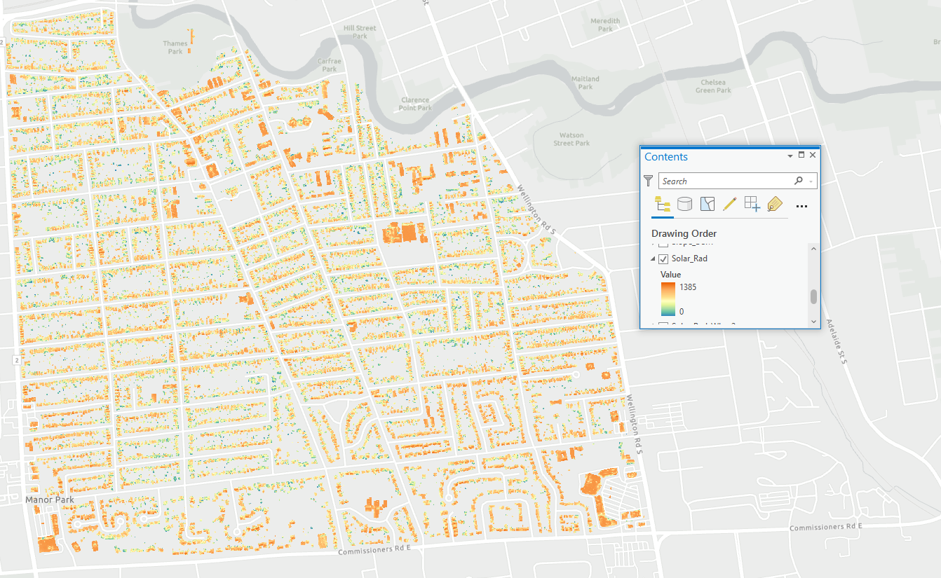
Step 3: Create a Solar Radiation Layer

The Area Solar Radiation tool in ArcGIS Pro is a powerful tool that can compute the total amount of incoming shortwave radiation based on the position of the sun throughout the selected time period, slope, elevation, and orientation of the surface. It’s incredible to me that this tool was able to compute radiation on a 1-hour interval, and checking 16 directions around each cell to identify light-blocking obstacles, using the input DSM layer for elevation data and latitude correction. These measurements would have been very difficult and nearly impossible without the assistance of computer models. In my previous project, I used Won’s (1977) hourly global solar radiation model to calculate the total amount of incoming shortwave radiation(K↓), it was relatively time consuming consider that there were many factors needed to be included, such as the cloud cover of the day, transmittivity of the radiation due to scattering from dust and dry air molecules, and absorption from water vapour. The result was also limited to a 2D satellite view only, I wasn’t able to include obstacles that may block the distribution of radiation over the surface (i.e. the sky view factor). This tool is so powerful in a way that it can compute in a 3D environment, capable of handling data from a long time period, and most importantly, has included the diffuse component of radiation as well as the idea of transmittivty.

“Transmittivity is a property of the atmosphere that is expressed as the ratio of the energy (averaged overall wavelengths) reaching the earth’s surface to that which is received at the upper limit of the atmosphere (extraterrestrial). Values range from 0 (no transmission) to 1 (complete transmission). Typically observed values are 0.6 or 0.7 for very clear sky conditions and 0.5 for a generally clear sky.”

With the data I input into this tool, the process took about 40 mins from start to finish, and I was able to get a complete solar radiation layer for my study area. I also used the Raster Calculator to convert the original unit KWh to MWh so it’s more readable.

Step 4: Identify Suitable Rooftops

The solar radiation layer only reveals the spatial distribution of the incoming sunlight (shortwave radiation). It’s important to know that not all roofs are suitable for solar panels, even though they may have enough supply of energy from the sun. There are three main criteria for a suitable roof and this is how they can be applied within ArcGIS:

1. Must have a slope of 45° or less because steep slope receives less sunlight.

For this, I used the Surface Parameters tool to create a slope raster layer from the DSM (I named this “Slope_DSM”).

Next, I used the Con tool to filter out cells that do not meet the condition where the VALUE of “Slope_DSM” is less than or equal to 45. This returns a raster that contains only values for cells that only a slope of 45° or less, all other cells are left out. I named this new raster “Solar_Rad_S”.

2. Must be able to receive at least 800 KWh/m² annually

I used the Con tool again to limit cells to those where the VALUE of “Solar_Rad_S” is greater than or equal to 800. This produces a raster that contains only the cells that have 800 KWH/m² or more. I named this “Solar_Rad_S_HS”, and it contains values for cells that have both low slow and high solar radiation.

3. Must not be facing north (north-facing roof receives less sunlight)

Finally, I used the the Surface Parameters tool to generate an aspect layer from the DSM. This creates a new raster that indicates the orientation of all cells within the raster, and I named the output from this “Aspect_DSM”.

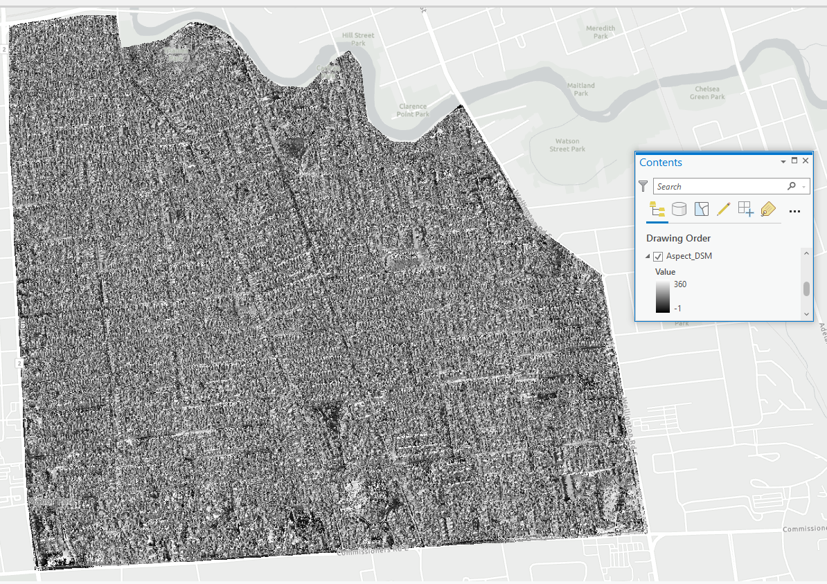
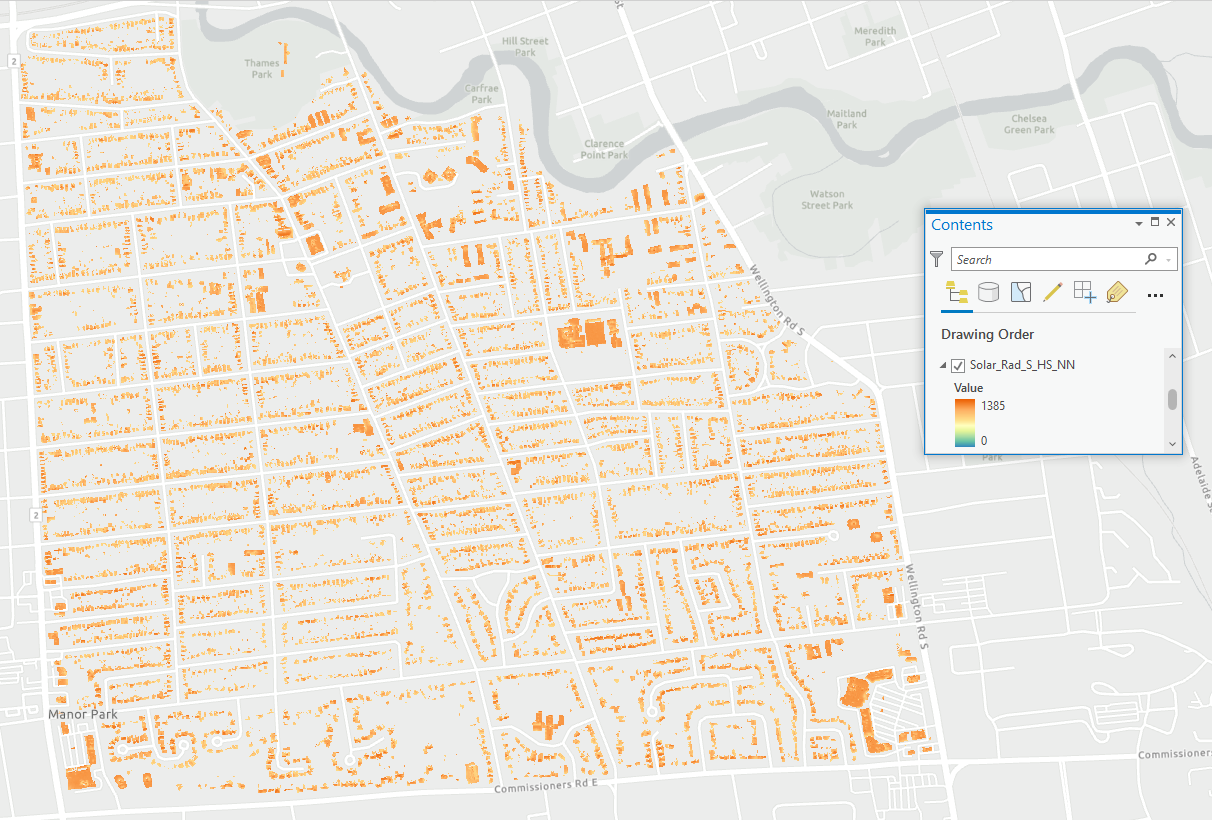
The “Aspect_DSM” layer can be used to create our final raster layer that I named Solar_Rad_S_HS_NN, revealing cells that have low slope, high solar radiation, and no north-facing aspects. This was accomplished using the “Con” tool to exclude cells that are facing north by filtering the raster data where the VALUE of “Aspect_DSM” is greater than 22.5, AND the VALUE of “Aspect_DSM” is less than 337.5.

Step 5: Calculate Solar Radiation and Electric Power per Building

Because our primary focus is on how much power can solar panels provide to each building, the map itself doesn’t know which cell belongs to which building, we have to group them together using the building footprint as a “mask”.

To do this, we can use the Zonal Statistics as Table tool, and before doing this, we need to use an attribute in the “Solar_Rad_S_HS_NN” raster that originates from a unique identifier in the “Building Footprint” shapefile. In this case, I had “OBJECTIVE_ID1”, so I used this as my “Zone_Field” with “Building_Footprint” as the feature zone data, “Solar_Rad_S_HS_NN” as the input value raster, and a statistic type of Mean. The output creates a table that I named “Solar_Rad_Table”.

Because we want to visualize the data inside the table, we have to join the table back to our “Building_Footprint” shapefil, using the Join Field tool (transfer Fields: AREA, MEAN). Now the “Building_Footprint” contains all the data we need:

• Building_ID (unique value assigned to each property)
• AREA (area covered by suitable cells in m²)
• COUNT (number of suitable cells per building, each cell is 0.25m²)
• MEAN (average solar radiation each suitable cell receive in kWh/m²)

We can continue to add two more fields called “Usable_SR_MWh” and “Elec_Prod_MWh” to calculate the usable solar radiation per building and how much of the radiation can be coverted into eletricity to power the house.

To measure total power available in Megawatt Hours, “Usable_SR_MWh” can be calculated as: “Usable_SR_MWh” = (AREA X MEAN )/1000

If we are assume solar panels only have a 15% efficiency, and only 86% of this converted power can be preserved in the system (according to United States Environmental Protection Agency (EPA)), then “Elec_Prod_MWh” can be calculated as: “Usable_SR_MWh” x 0.15 x 86

Now we have all the information we need to visualize the final outputs, and make a final assessment of the selection criteria we used. In this case, there are three criteria still need to be addressed:

1. The roof needs to be at least 30 m² in size to meet the installation requirement of solar panels.
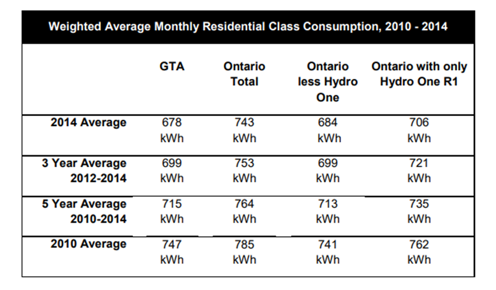
2. Average household in Ontario uses 9.17 MWh per year (based on the 5-year average monthly consumption data in Ontario is 764 kWh (in the table below); 764 kWh * 12 months / 1000 = 9.17 MWh per year). This means a roof needs to be able to generate electricity of more than 9.17MWh on an annual basis to be deemed as “suitable”.
3. Cost of installation and maintenance.

These two criteria can be easily applied using the Select by Attribute tool to select buildings from the data where “Area”> 30 AND “Elec_Prod_MWh” > 9.17. I exported these features to a raster that I called “Suitable_Cells”. My last approach was a little bit different than what’s being taught in the lesson plan because we have different statistics in electricity consumption. For the third criteria, I’m thinking I will create a web app that can embed a cost calculator on the side so that people can quickly get na estimated cost for switching to solar power, and decide whether or not to stay on existing power grids.

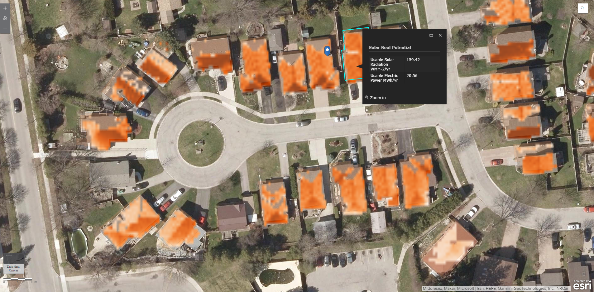
I was also able to share my ArcGIS Pro files online and made an interactive Web map using ArcGIS Online, using the two shapefiles and one raster file (which I uploaded as a hosted layer in KML format). This online map offers several useful features such as:

1. Look up addresses
2. Zoom in to inspect individual property
3. Switch to a satellite imagery base map to see where approximately solar panels can be installed over the roof.
4. The pop-up tells you the solar potential of your roof in terms of useable solar radiation, and the possible electricity it can generate.

Conclusion

Before starting the project, my hypothesis was that over 90% of homes in Wortley Village/Old South should be suitable for solar roofing because a majority of the properties in this neighbourhood are relatively large, detached single family homes. It was reasonable to expect that every house facing south was suitable to have solar panels installed over their roof. However, the results from my project rejected my hypothesis. There aren’t as many houses suitable due to a variety of constraints, such as high slope of the roof restricts the amount of receivable shortwave radiation, the size of the suitable areas being too small to generate enough power, and limited sunlight hours due to orientation and elevation of roofs. The combination of the “Area Solar Radiation” tool in ArcGIS Pro and the LiDAR-derived DSM provide an efficient method to quickly analyze the solar rooftop potential of a community. Having this dataset available online also allows me to continue further by sharing the results with those who are interested within the local community, who may benefit from having access to the results of a GIS analysis like this.