Uncovering the Power of Remote Sensing in Micrometeorological Studies

In my third-year micrometeorology class with Dr.Voogt, we were assigned a course project to work in small groups throughout the term, and each group had to conduct a research project for related to microclimate or micrometeorology. The course covered a wide range of topics such as solar radiation budget, soil microclimates, surface temperatures, etc. For our project, we primarily focused on solar radiation and energy balances, using the City of London as our study area to examine how each of the radiation and energy balance terms vary across the region in a specific time.

Since my partner and I have prior knowledge in remote sensing and GIS, we decided to use existing Landsat 8 data, instead of going out to collect data in the field.  We haven’t yet done any research in the field of urban microclimate using GIS, thus I wanted to share some of the steps and methods we used in our project for anyone who may share similar interests. The project was very challenging because it involved applying a lot of concepts from our course and doing a lot of calculations both within and outside of ArcMap. I found that it’s very helpful to map your thoughts in a flow chart first before doing anything, because having a chart on hand will certainly reduce the chances of meeting a dead end, and it can provide a sense of whether the project is feasible with your level of experience, the amount of data that is available, and the time that you have.

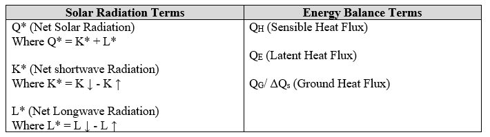
For summary, we were using Landsat 8 and ArcMap to generate raster layers for these terms:

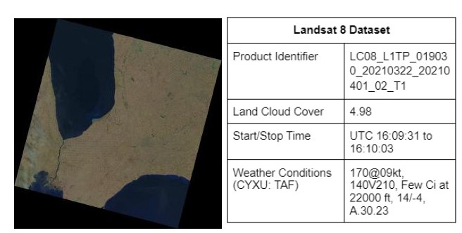
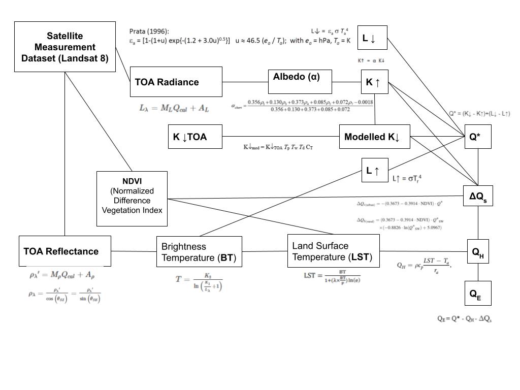
We chose Landsat 8 to acquire our dataset given that its 30m resolution and 11 spectral bands were adequate for our study area. The attached pictures are a quick snapshot of the dataset that we used, and a flow chart of how each raster layer was generated.

K ↓ (Incoming Shortwave Radiation)

We chose a physically-based solar radiation model by Won (1977) to calculate an estimate value of K↓:

K↓_TOA = K↓_EX = S₀ cos Z

K↓= K _MOD↓ = K↓_TOA T_p T_w T_d C_T

For our study date and using the data from CYXU Weather Station (at the London airport), our calculations show that incoming solar radiation: K↓ = 979.639 W m^-2

Reference: Won, T. K., 1977: The simulation of hourly global radiation from hourly reported meteorological parameters—Canadian prairie area. Proc. Third Annual Conf., Edmonton, AB, Canada, Sol. Energy Society of Canada

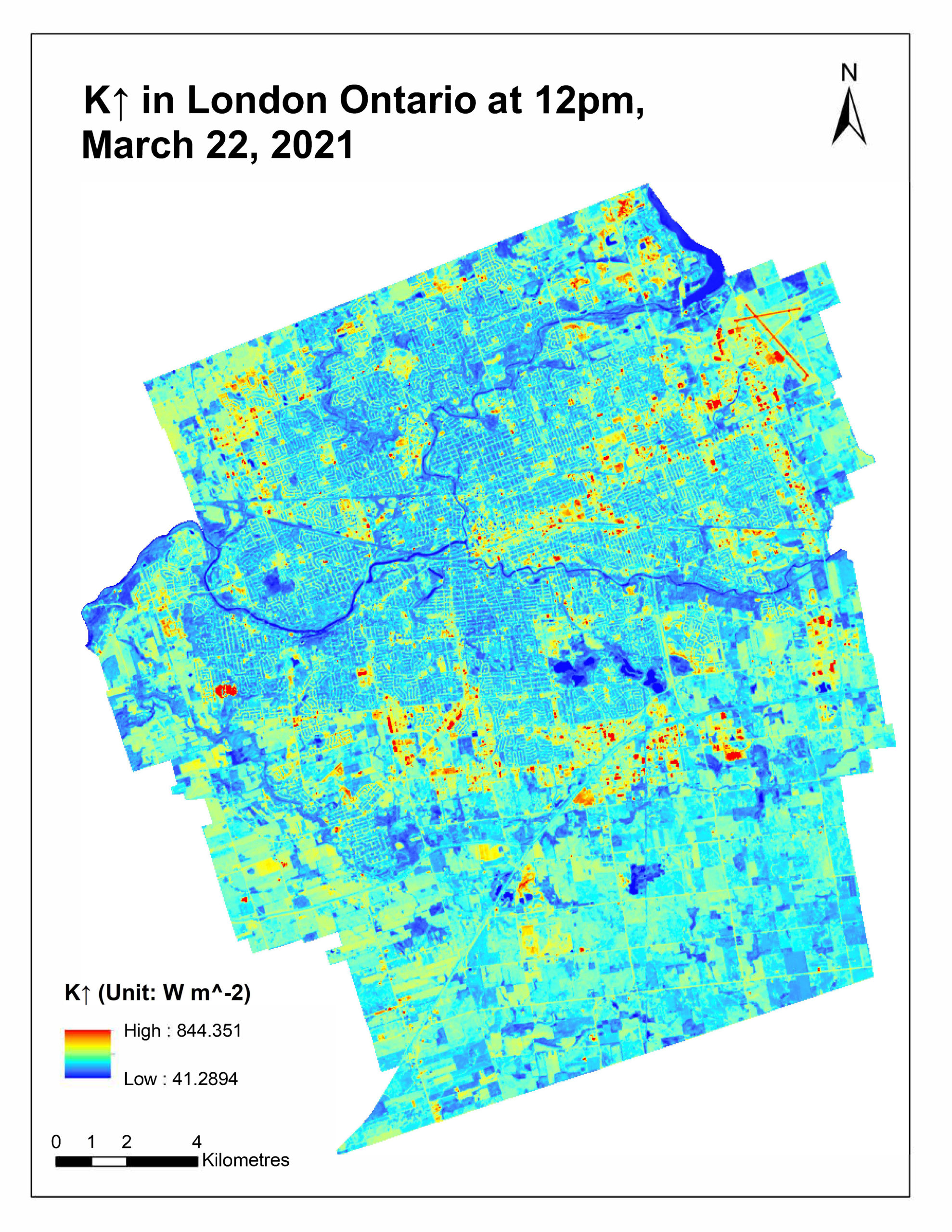
K↑ (Outgoing Shortwave Radiation)

To calculate K↑, there were three steps involved.

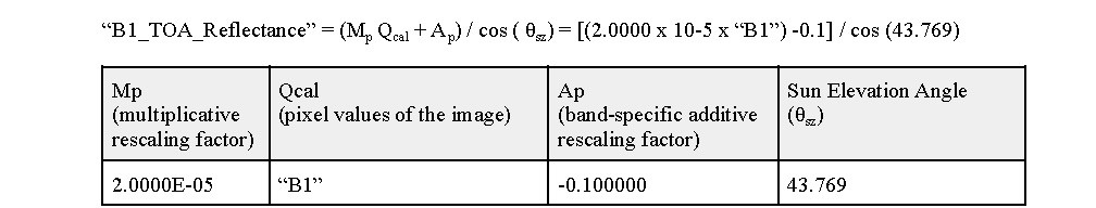
First, we need to convert the digital numbers (DN) in the Landsat 8 Dataset to TOA Reflectance (Top of the Atmosphere) for Bands 1, 3,4,5, and 7 according to the instructions from USGS.

To demonstrate:

Second, we need to determine the albedo of the surface (i.e. the ability of surface to reflect radiation) using Liang (2000) and Smith (2010)’s methods in their journals. To generate the “Albedo” layer in ArcMap, this formula was used:

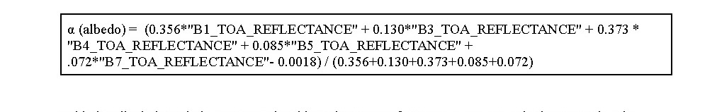
Third, after getting the albedo layer, we can quickly generate the K↑ layer knowing that K↑ = K↓ x albedo.

L↓ (Incoming Longwave Radiation)

With a similar approach as calculating K↓, we modelled the amount of L↓ using Prata’s (1996) method to estimate apparent atmospheric emissivity (ε_a) using the hourly air temperature, and vapour pressure from the CYXU weather station.

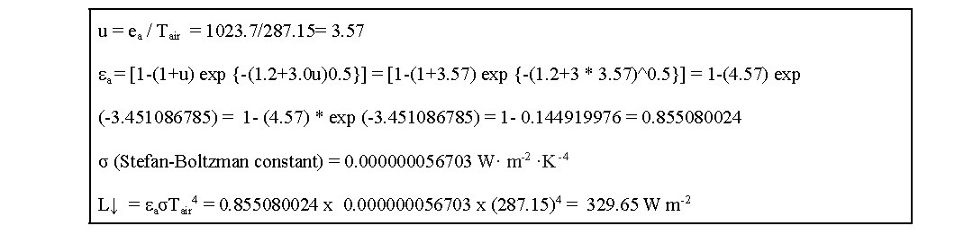
Reference: Prata, A. “A New Long-Wave Formula for Estimating Downward Clear-Sky Radiation at the Surface.” Quarterly Journal of the Royal Meteorological Society, vol. 122, no. 533, 1998, pp. 1131

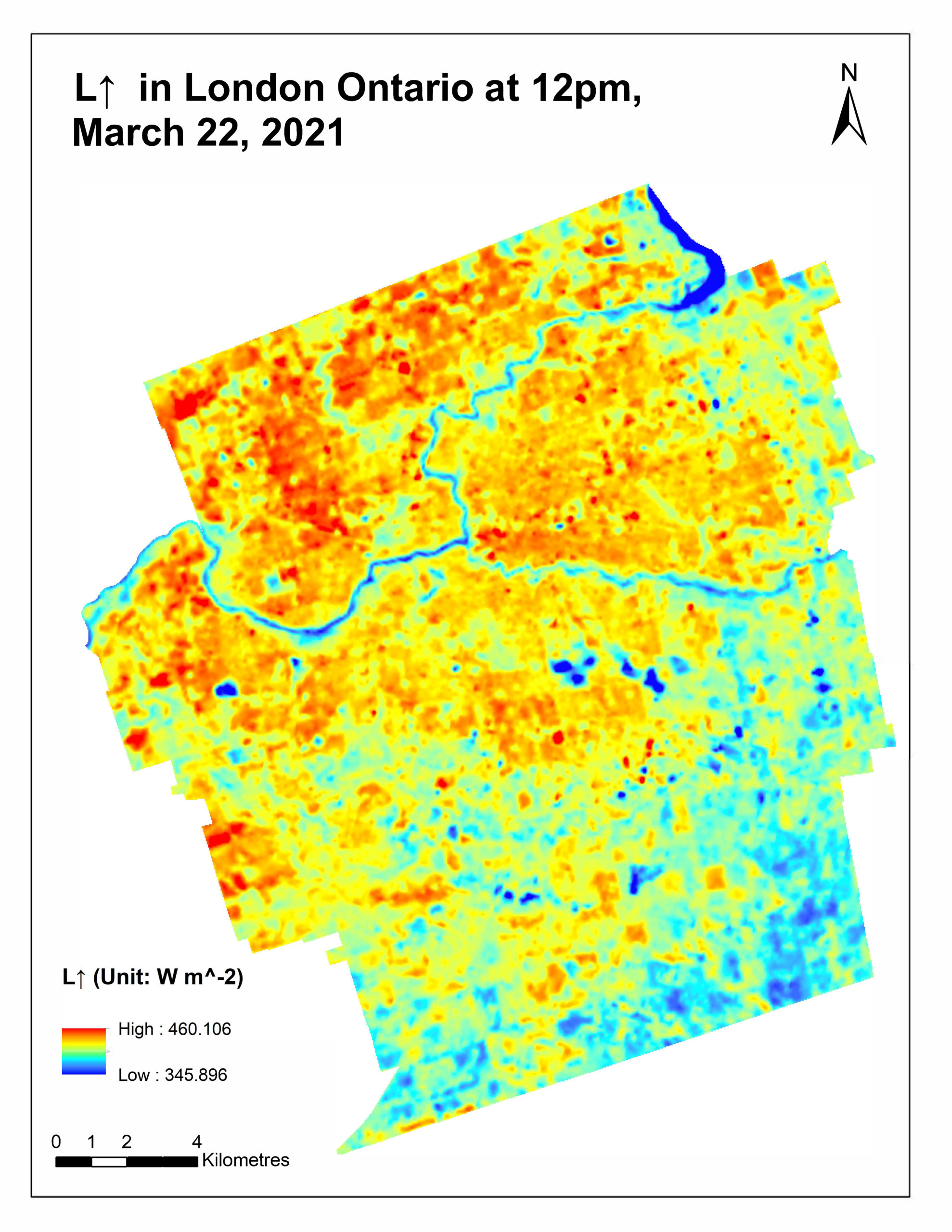
L↑ (Outgoing Longwave Radiation)

Similar to K↑, there were three steps in getting L↑.

Firstly, we need to generate a layer for “TOA Radiance” (spectral radiance at the top of the atmosphere observed by the satellite) using the Band 10 in the Landsat 8 dataset, according to the instructions from USGS.

To demonstrate:

Secondly, we need to convert the “TOA Radiance” to “TOA Brightness Temperature”.

For our case, we have:

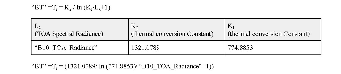
Thirdly, we need to apply the equation L_↑  = σ T_r⁴ , and we can rewrite the equation as L↑ = σ T_r⁴  = 0.000000056703 x (“BT”)⁴  in the raster calculator.

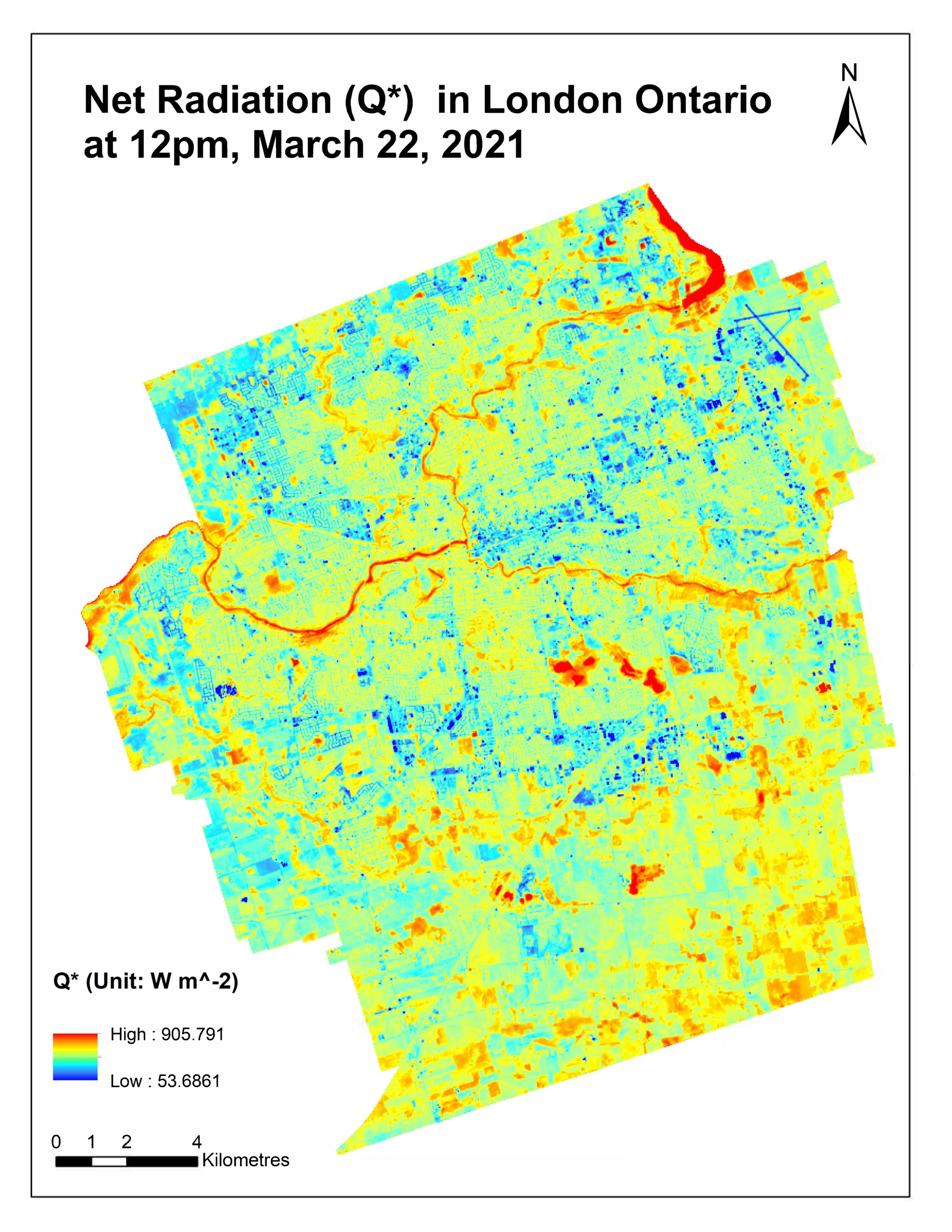
Q* (Net Solar Radiation)

After layers of K↑, K↓,  L↑, and L↓ have been generated, we can easily generate Q* knowing that Q* = (K↓- K↑) + ( L↓- L↑). As soon as we had Q*, we proceeded to the next stage of our research, which was to determine the energy balance terms (ΔQs, Q_H and Q_E).

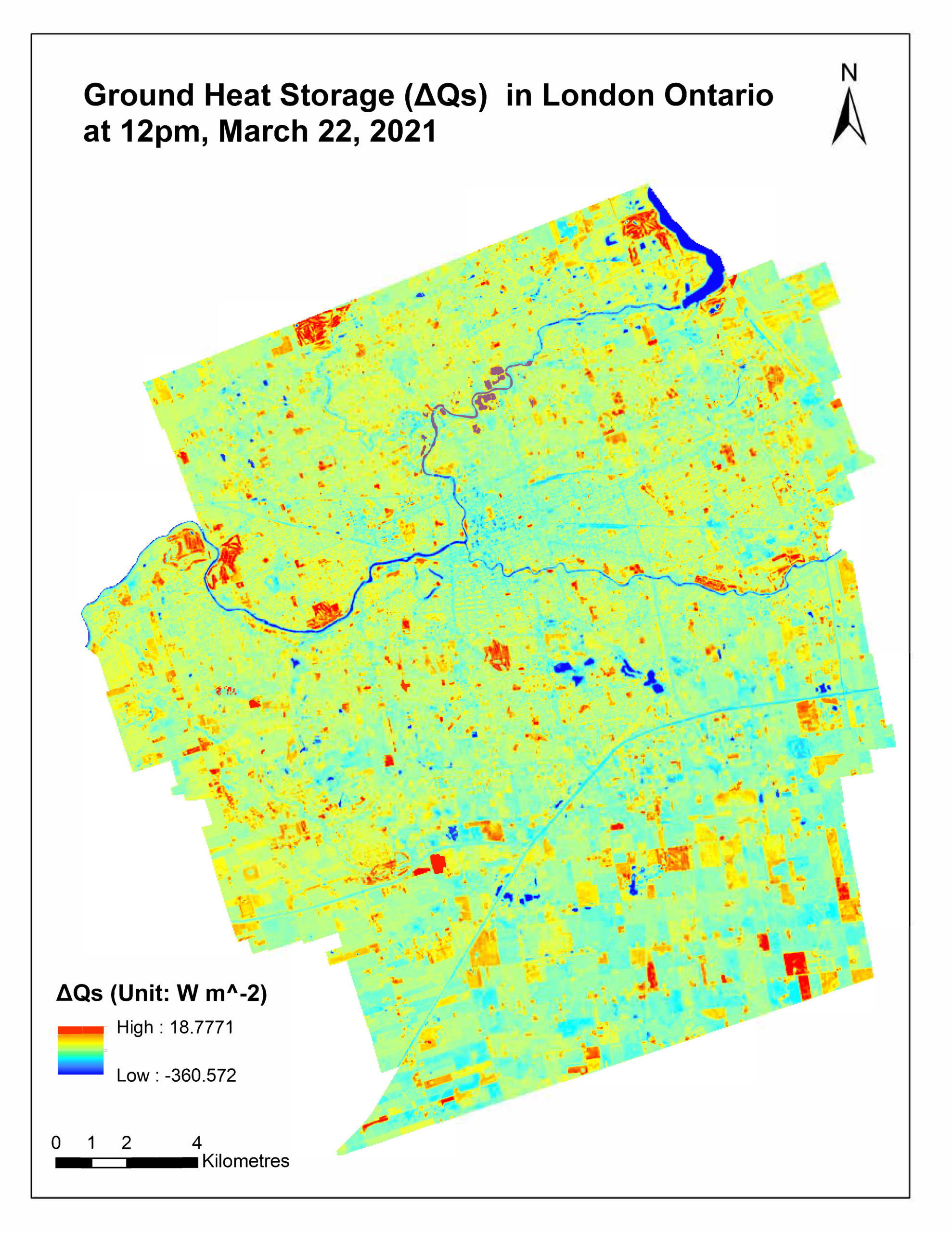
ΔQs (Storage Heat Flux or Ground Heat Flux)

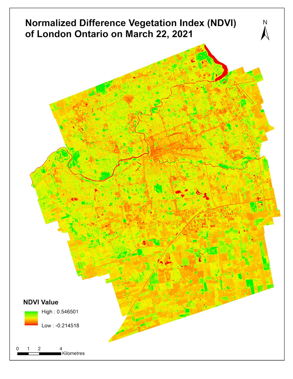
Rigo & Parlow’s paper in 2007 provides three methods to extract ΔQs in an urban environment, we chose the “NDVI Approach” for our research because generating a NDVI layer is relatively easy in ArcMap using Band 4 and 5 from Landsat 8.

NDVI = (NIR-RED)/(NIR+RED) =(Band 5 – Band4) / (Band 5 + Band 4)

The NDVI Approach works by assuming that vegetation reduces ground heat flux (ΔQs)  because much of the heat is transformed into latent heat flux, thus higher NDVI value leads to lower ΔQs. Since Rigo & Parlow’s method divides ΔQs into two separate categories (urban vs. rural), we need to use the NDVI value as our filter to create a formula that can combine these two layers into one, for our case, we used:

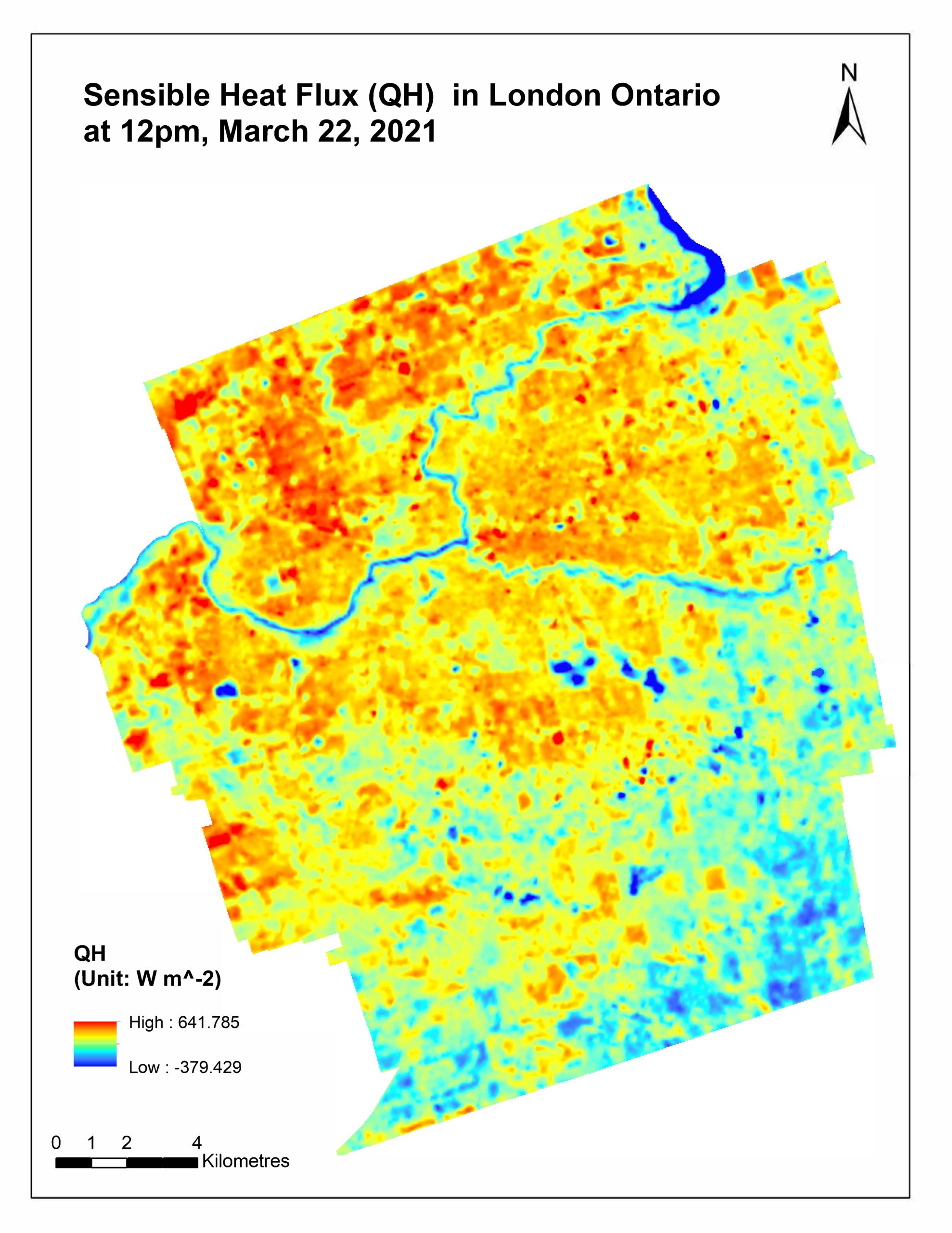
Q_H (Sensible Heat Flux):

Parlow also had another paper in 2018 that provides a method called “ARM” (Aerodynamic Resistance Method) to derive Q_H from satellite images with limited data.

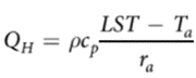
For our dataset, we have:

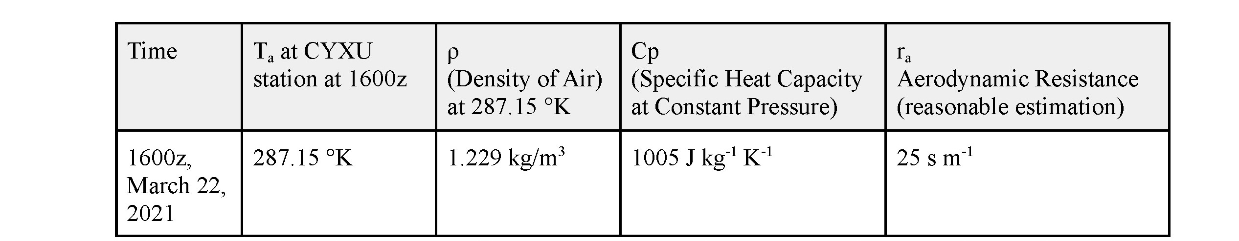
It’s important to take note that the value of aerodynamic resistance was a quick estimation, because the actual value varies spatially with displacement length, wind direction and wind speed on the ground if we were to calculate for every pixel.

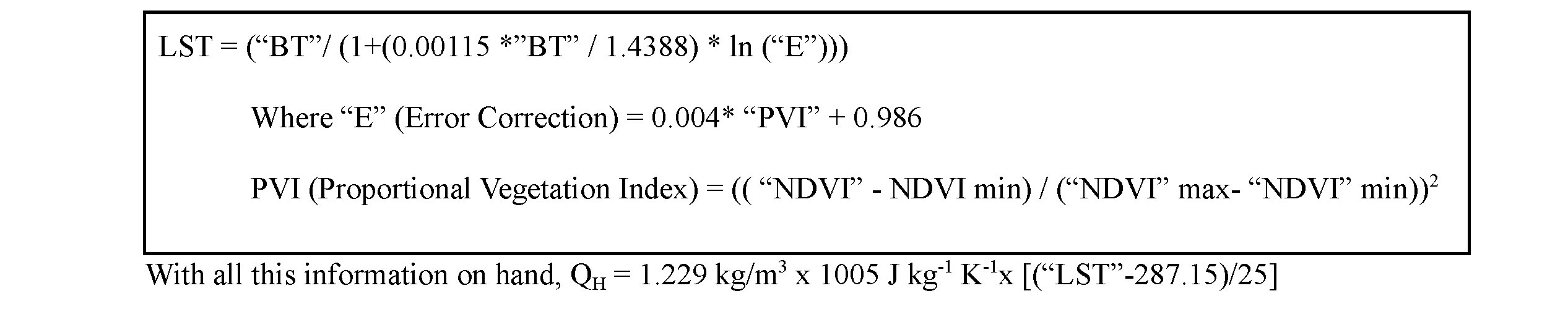
Land Surface Temperature (LST) can be obtained from the “TOA Brightness Temperature” layer in the previous steps, using Franzpc’s (2018) method:

Q_E (Latent Heat Flux)

            Q_E was very difficult to determine because we were dealing with a 3D non-homogenous environment, therefore we can’t simply apply the formula Q* = Q_H + Q_E + Q_G = Q_H + Q_E + ΔQs to generate this layer with shortcuts. For the extent of our study, we determined that Q_E was not a major topic of concern because we were able to use the other terms to conclude our analysis. Parlow (2018) provides a more advanced method to estimate Q_E although it would require collecting ground-based data. In the future, estimating Q_E with remote sensing technology can be possible if we have the needed equipment on the ground stations to combine with satellite data.