
Collecting and Calculating Land Data – Preparing for Analysis of Remote Sensing Microscale Urban Heat
A few months ago, I wrote a blog post introducing my MSc Thesis. Since then, I finished my summer fieldwork which consisted of cycling over 560 kilometres of cycling and road infrastructure measuring air temperature every 1-second in Mississauga, Ontario. I also had the opportunity to present my preliminary thoughts on this project at the International Medical Geography Symposium (IMGS) in June 2022.
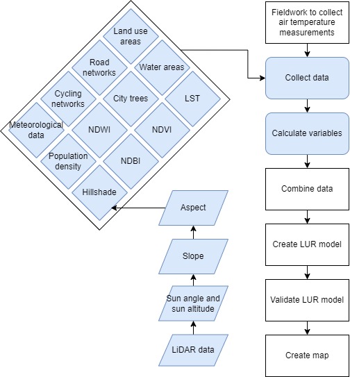
This study uses remote sensing and geographic information systems (GIS) to map microscale heat exposure by creating a land-use regression model to relate land surface temperatures to ground-level temperatures using remote sensing satellite data and other land variables. Regarding current progress, I completed calculating the land use variables within buffers (5m, 25m, 50m, 100m, 200m, 400m, 800m, 1600m) or distance to object for the land-use regression model. I selected points from every 1-minute of my cycling fieldwork, then created buffers around each point. Then, I will create a micro-scale map representing heat in Mississauga. In this blog post, I will review the data and data sources I have used for this project so far.
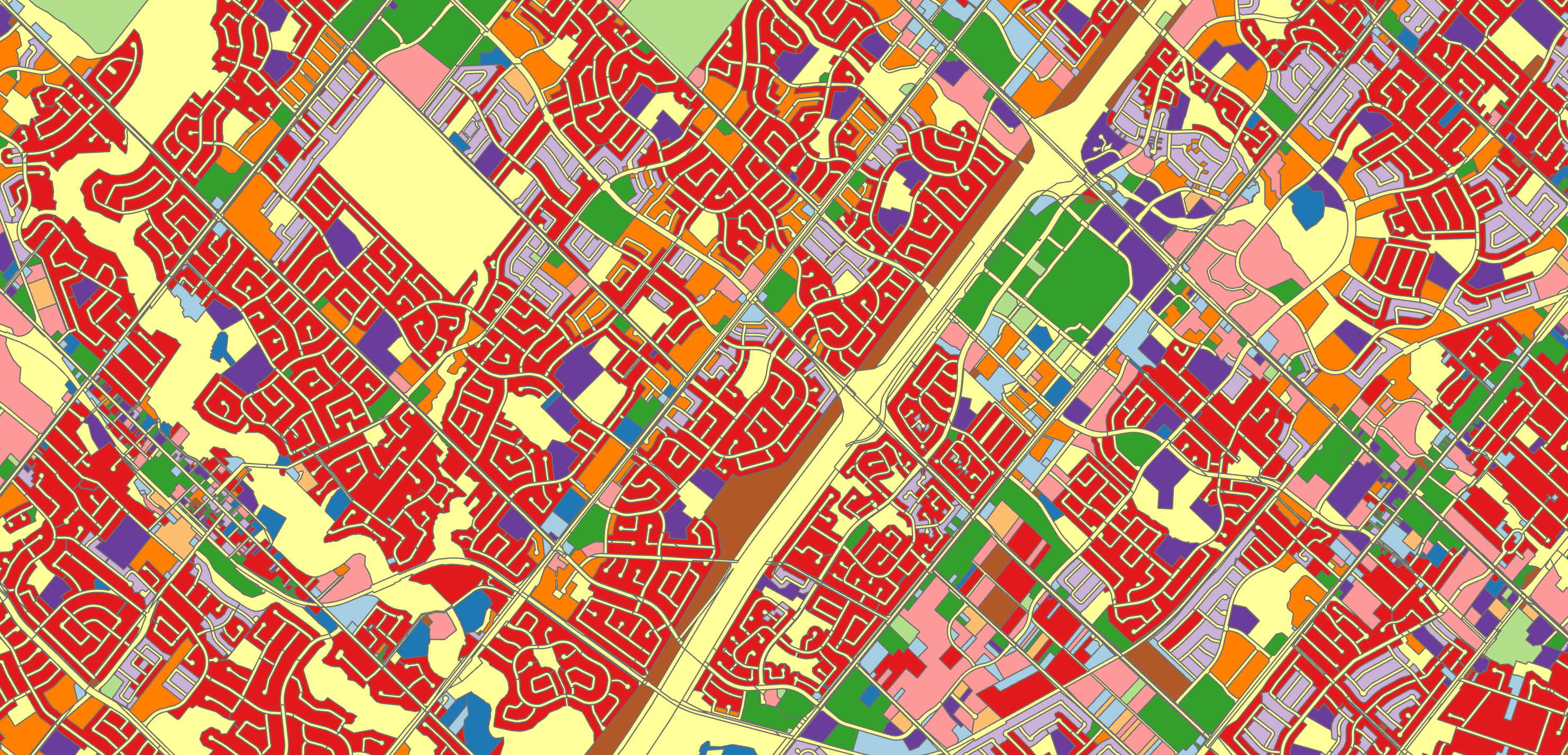
First, I obtained detailed existing land use data from the City of Mississauga open database, and I calculated the total area within each buffer. The data included land uses such as Residential Detached area, Industrial General area, Office area, and Farm area. The land-use data covered all of Mississauga, defining every piece of land.
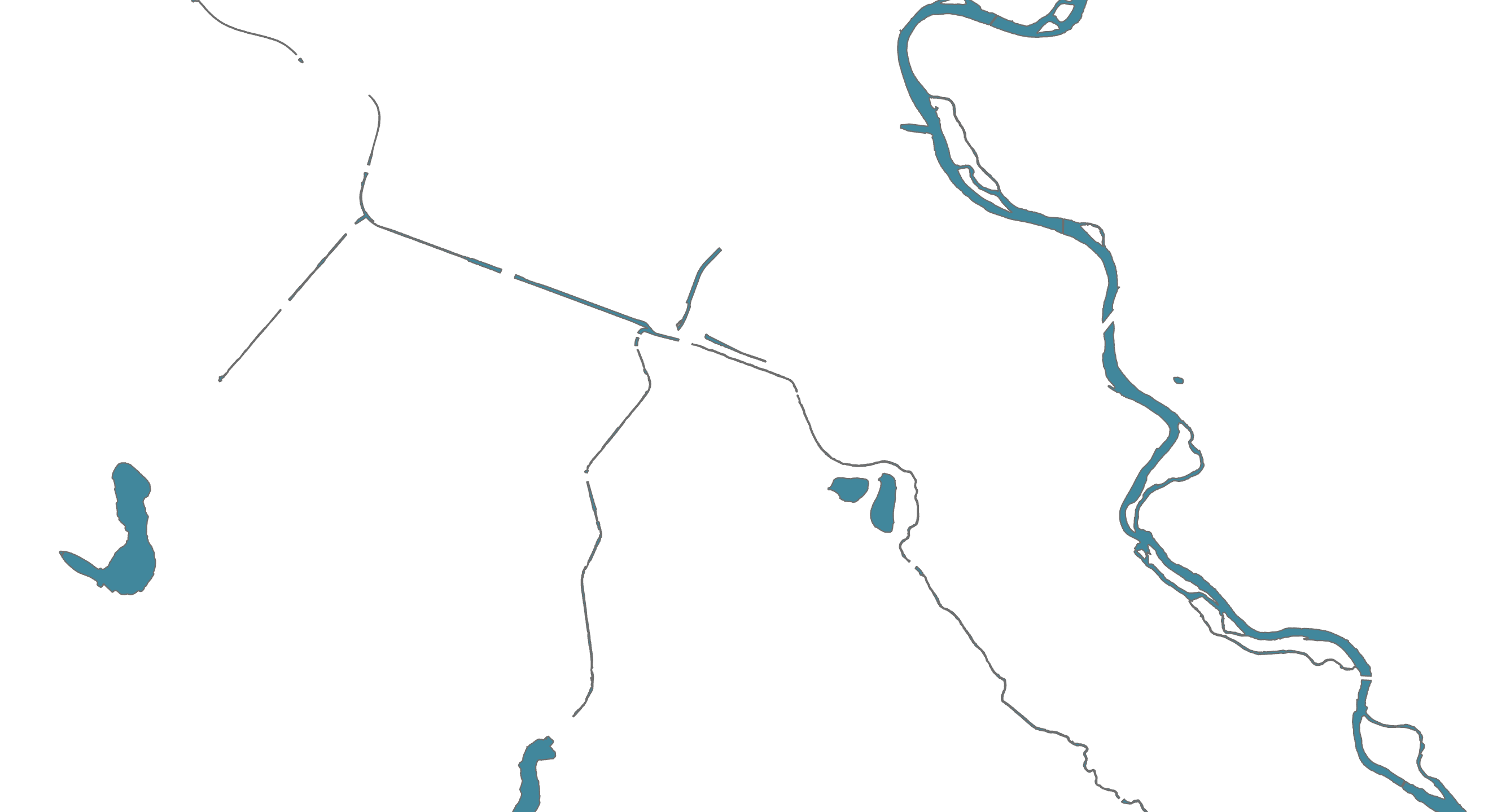
The above land-use data did not account for water areas, which I obtained from Scholars GeoPortal. I calculated the area with each buffer also.
In addition to land data, I also obtained census road networks and cycling networks from Statistics Canada and the City of Mississauga, respectively. I obtained information on roads, such as primary highways, local roads, and bridges/tunnels. Every official road in Mississauga was defined in the data. My cycling fieldwork also consisted of cycling on roads and bicycle paths, which is why I also accounted for cycling network data, such as buffered bike lanes, multi-use trails, and off-road trails. Every official Mississauga cycling route/path was included in the cycling network data. The road and cycling data were calculated by distance to the object.

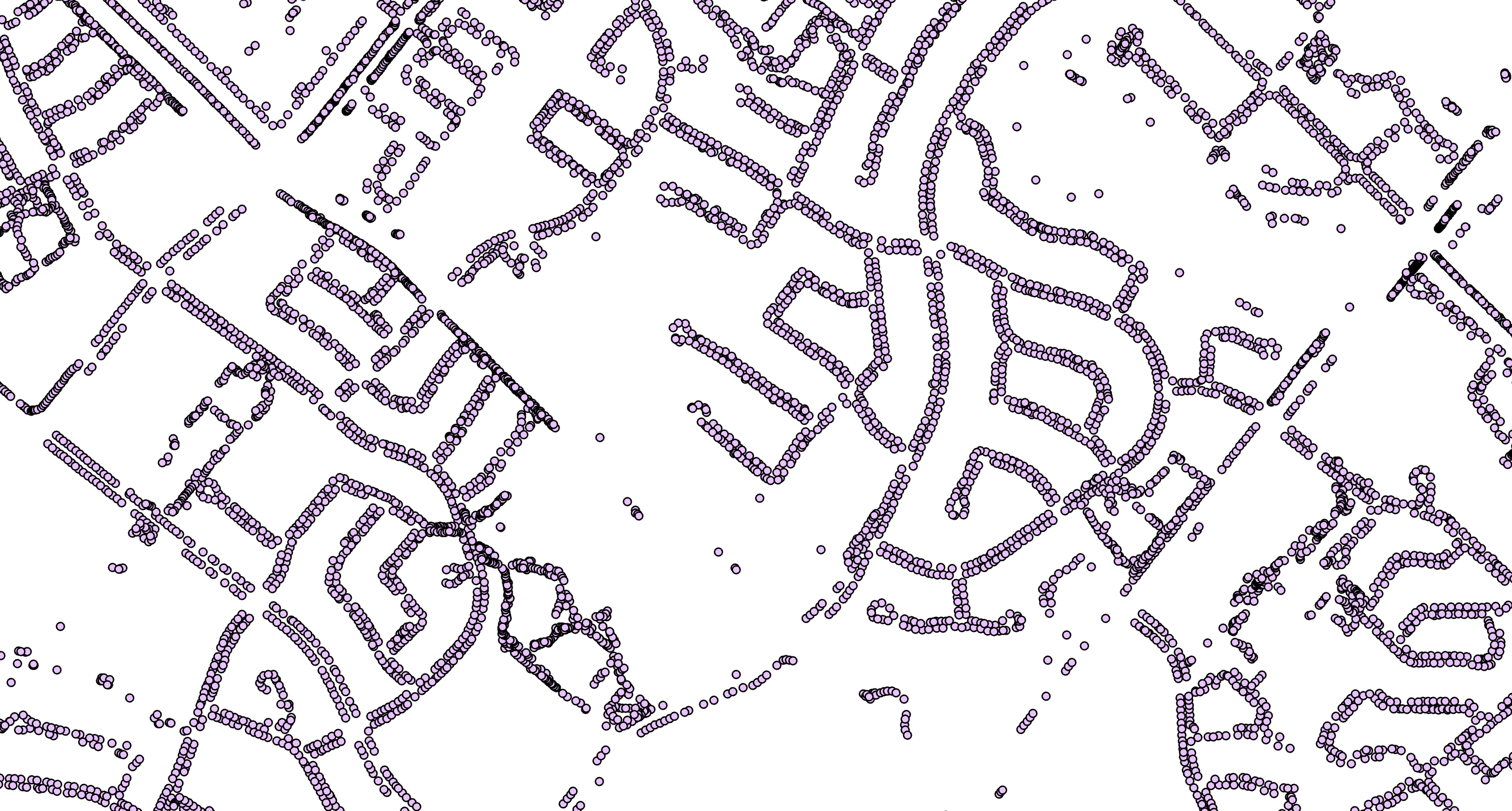
I obtained city tree data from the City of Mississauga. I calculated the number of city trees within each buffer and the distance to the closest city tree.
Indices such as Normalized Difference Vegetation Index (NDVI), Normalized Difference Built-Up Index (NDBI), and Normalized Difference Water Index (NDWI) were also calculated and considered. I obtained these data from Google Earth Engine, by merging USGS data from satellites Landsat 7, 8 and 9. I calculated the average NDVI, NDBI, and NDWI within each buffer.
I obtained a course land surface temperature (LST) also using Google Earth Engine by merging MODIS Aqua and Terra satellites. I extracted the LST from each point.
I obtained meteorological data from Pearson International Airport containing hourly temperature, hourly dewpoint, hourly relative humidity, hourly wind direction, hourly wind speed, hourly visibility, and hourly air pressure.
I calculated population density by obtaining population counts from Computing in the Humanities and Social Sciences (CHASS) at the University of Toronto by Forward Sortation Areas (FSA) and the area from Statistics Canada Census Boundary by FSA.
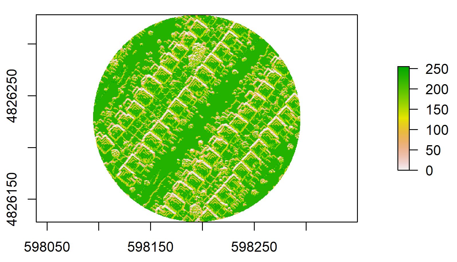
The most difficult part of the project was conducting a shadow analysis. First, I received LiDAR data from the City of Mississauga in small tiles in laz format. I used the Convert Las tool in batch in ArcGIS Pro to convert the laz files to lazd, to be compatible with ArcGIS Pro. Then, I merged all the lazd files using the Create Las Dataset tool. Then, to make the data easier to interpret and prepare for later analysis, I converted the lazd file to raster using the Las Dataset to Raster tool at 0.5 meters. Finally, I converted the raster values to integers and clipped the raster perfectly to Mississauga. I managed to obtain sun position data, including the sun angle and sun altitude, by using the suncalc package in R, which allowed me to collect the sun angle and sun altitude for every minute of my cycling fieldwork. The sun angle and sun altitude depended on the location, date, and time of each point. Then, to determine if each point was in shadow or no shadow during my fieldwork, I created a hillshade for each point using the hillshade function in R. First, I needed to obtain slope and aspect rasters done in ArcGIS Pro. Then, I was able to create hillshade rasters to then extract the hillshade values that range from 0 to 255. Values above 0 indicate no shadow and light intensity, and values of 0 indicate shadow.
And there we have it! The next steps are to create a land-use regression model to map heat across the entire city of Mississauga, Ontario.
Thank you!
— Scarlett Rakowska