
Computational method of ArcGIS Ordinary Kriging tool
ArcGIS provided outstanding and friendly interpolation tools to common users. I unitized Kriging tool in ArcGIS to interpolate the data points a long time ago. However, understanding its method is a different story. My previous background is in Applied Geology, particularly Groundwater modeling. I, therefore, had a chance to learn the meaning of the ArcGIS Kriging method through Stochastic Subsurface Hydrology class. I would like to share a very basic computational method of the Ordinary Kriging technique which is used more popular for the interpolation of point data.
Kriging is applied for the first time by a South Afrikaans engineer Krige to estimate gold concentrations in ore deposits. This technique is known as an estimated surface produced by the sophisticated geostatistical technique from a dispersed collection of points with z-values. It is a powerful tool in ArcGIS Spatial Analyst geoprocessing toolbox that could be applied to different scientific fields.
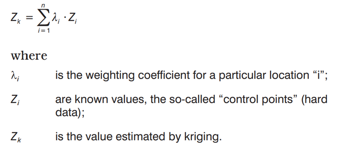
Ordinary Kriging estimate unknown value of a regionalized variable (Zk) by surrounding known values (Zi) based on weighted coefficient for a specific location (i).
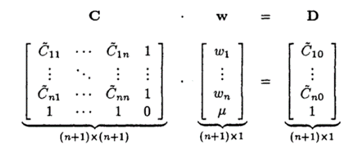
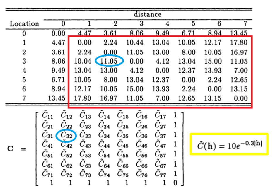
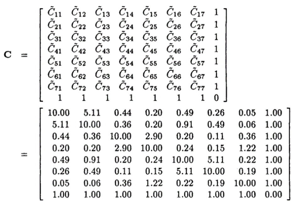
This general formula can be written as the matrix equation that their value is presented as variogram values.
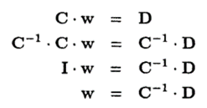
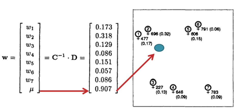
To get easier for solving the weight variable, an invertible step is carried out as below.
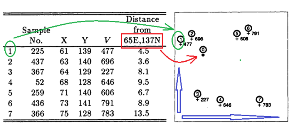
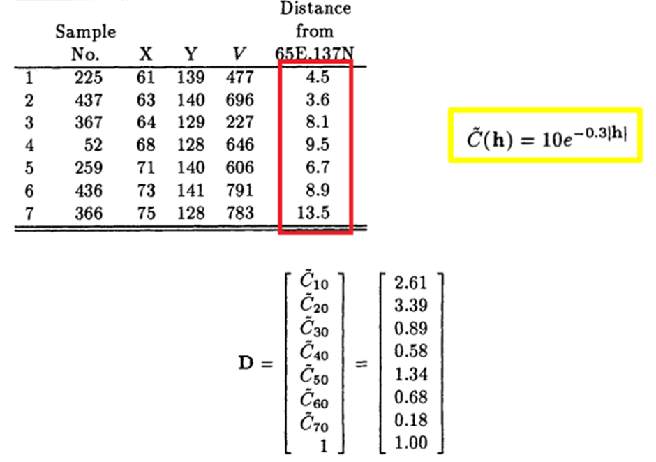
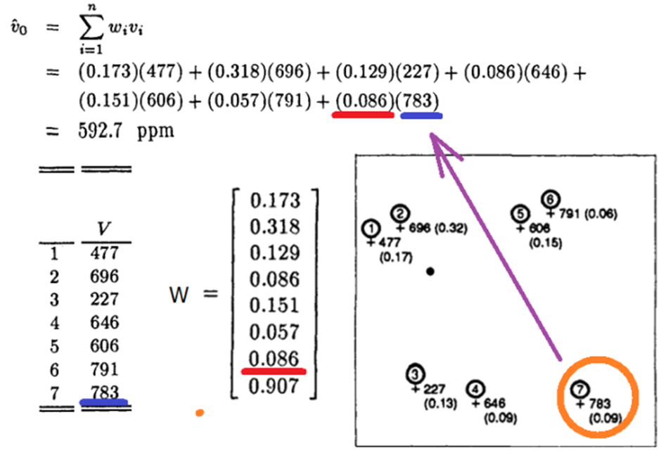
In this example, we have to find the real value of an unknown value, and it is the value of position number 0 in this case. As you can see in Figure 3, we have the value of data points of 1 – 7 except 0 position – an unknown point. The only thing we have known is 0 point location. Since then, we can calculate the distance from surrounding known points to this unknown point and another points as well.
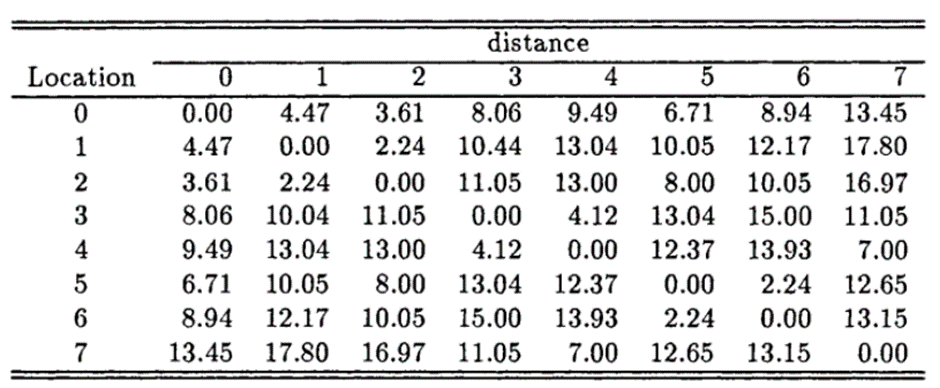
Because the dataset has its own weighted value and impacts each other in the study area. A matrix expressed by variogram values is established.

Finally, to make the final results more accuracy, we should carefully consider factors such as control points, the sill, experimental variogram, variogram range, nugget effect, and Lagrange multiplicator should be carefully considered in this spatial model. Once we understand the relationship between these factors and the meaning of data trends, we can confidently choose the appropriate parameters in the Semivariogram table in the ArcGIS Kriging tool (Figure 11).
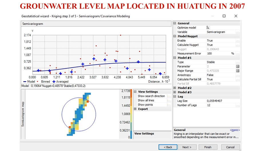
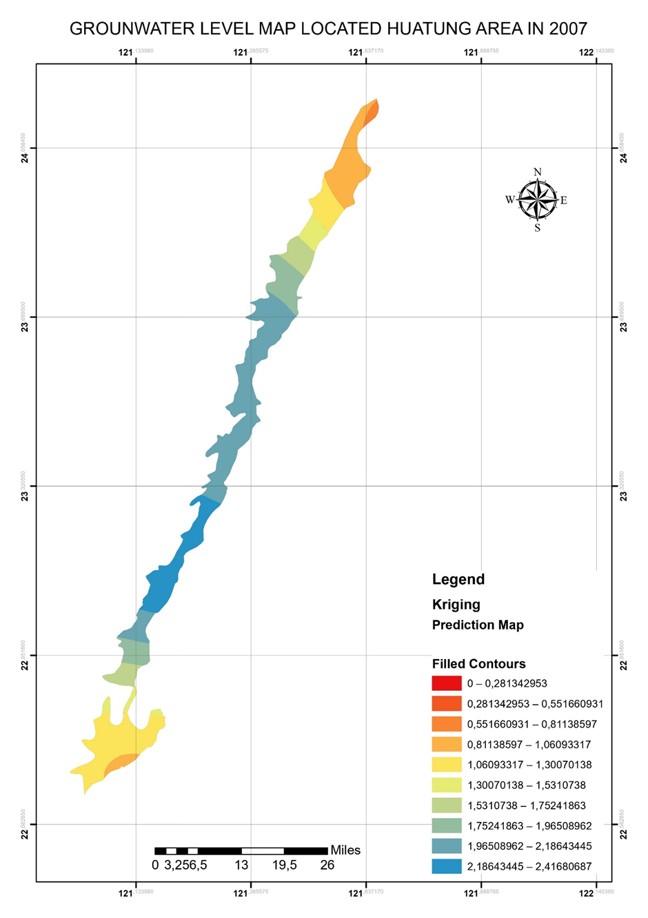
Figure 12 is a piece of example groundwater level maps I have conducted in my Stochastic class. The map is built by ArcGIS Geostatistical analysis tool based on a dataset collected in HuaTung, Taiwan.
NEXT STEPS
I am currently studying for MEng program in the Geodesy and Geomatic Engineering Department, University of New Brunswick. I am interested in Ocean mapping and Physical Oceanography. It would be a sharing of creating a bathymetric map by ArcGIS or ArcGIS Pro in the future when I have more chances to learn about this.
Hope this post has delivered some useful insights about spatial analysis. Enjoy!
REFERENCES
1. Professor Chuen – Fa Ni, Stochastic Subsurface Hydrology lecture, December 01, 2020.
2. Dr. Nguyen Hoang Hiep, Mini project – Kriging, December, 2020.
3. Edward, I., & Srivastava, R (1989). Applied Geostatistics. Oxford University Press.
4. Malviæ, T., & Baliæ, D. (2009). Linearity and Lagrange linear multiplicator in the equations of ordinary kriging. Nafta, 59(1), 31-37.