
Quality Assessment of the OpenStreetMap Road Network in Calgary, Alberta Using ArcGIS Pro Python Notebook
By rapidly growing the volunteered geographic information (VGI) platforms in recent years, accurate and up-to-date geospatial data are being provided more and more every day. Moreover, these open sources data are easily and freely accessible to the users. This creates a challenge for the various governmental mapping organizations which have well-established mandates to map the country. However, one important question is that are these VGI sources truly reliable? While coverage and accuracy of VGI cannot be guaranteed, still they contain information that could be beneficial for the official mapping organizations, and maybe there is a potential to create a bridge between these two worlds to get even more comprehensive information. But, before doing anything, we have to evaluate the overall reliability of VGI first.
OpenStreetMap (OSM) is a popular VGI platform that allows users to create or edit maps using GPS-enabled devices or aerial imageries. The issue of geospatial data quality in OSM has become a trending research topic because of the large size of the dataset and the multiple channels of data access. The objective of this project is to examine the overall reliability of the city of Calgary OSM data. The Built-in Python notebooks feature in ArcGIS Pro is very useful for creating and automating the process of assessing the quality of the OSM road network.
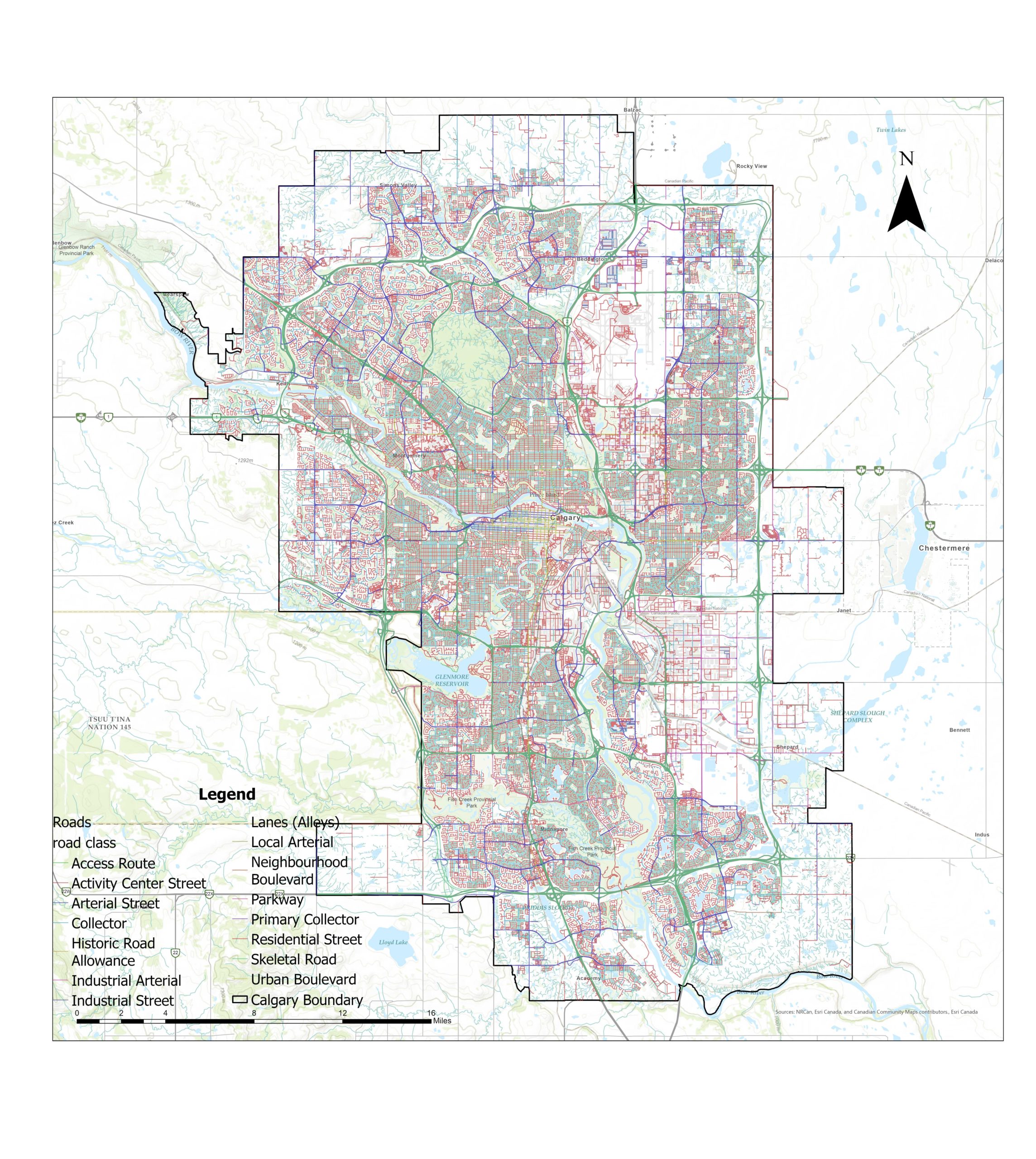
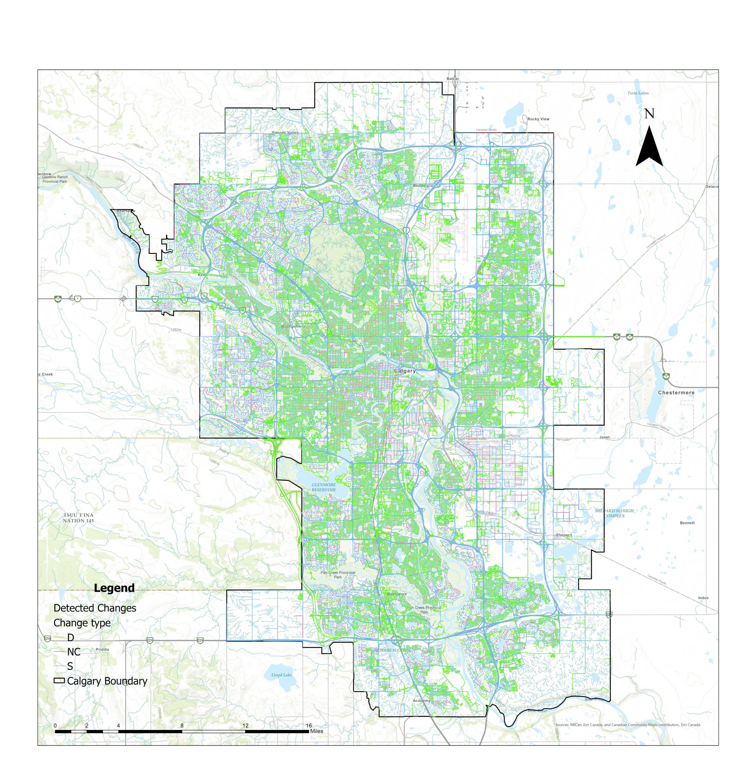
In the first step, I collected two datasets, one is the Calgary road network from the Calgary Open Data provided by the city of Calgary, and the other one is the OSM road network for the city of Calgary. The entire city of Calgary road map can be seen in Figure 1.
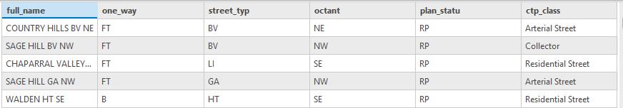
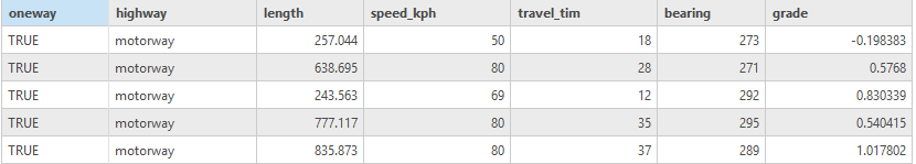
In Figures 2 (a) and (b), the attribute table of both datasets is shown. Both datasets contain different attributes which have the potential to be merged if the results of the quality assessment show that could be the case.
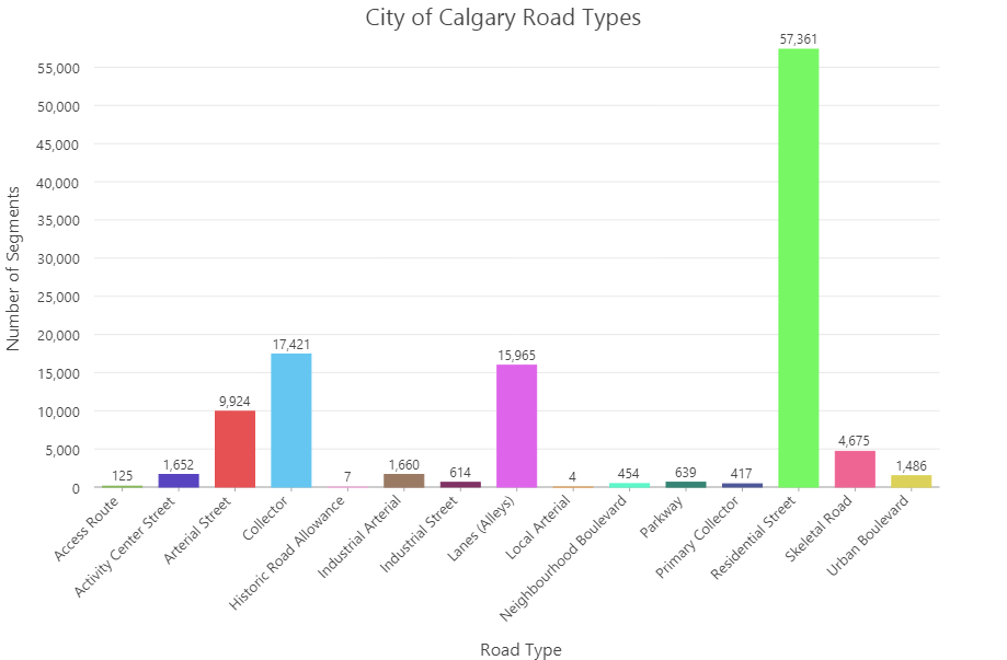
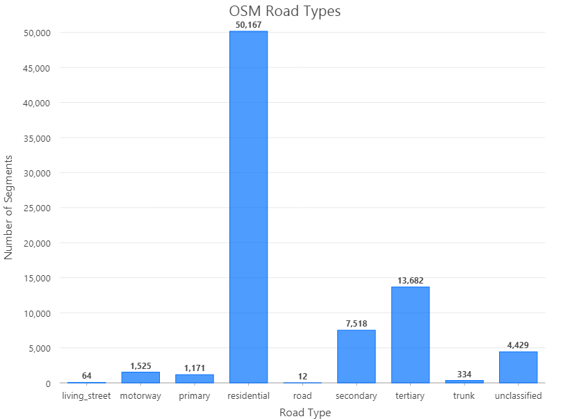
Figures 3 and 4 show the classification of road types in both datasets as well the number of segments in each category. It can be seen that both datasets have different classifications for their data.
Completeness
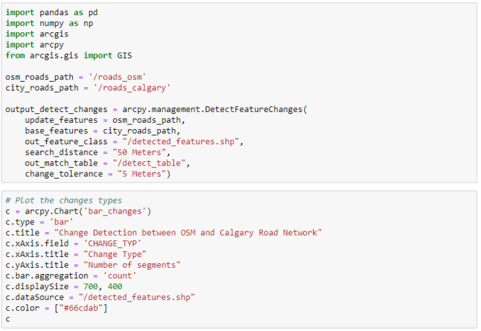
For evaluating completeness and positional accuracy, geometric feature matching was performed to identify unmatched road segments. This can be done by using the “Detect Feature Changes” analysis in ArcGIS Pro Notebook. Here in the next figures, part of the code which includes implementing the “Detect feature changes” as well as the results of the analysis are shown.
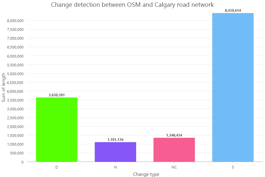
The bar chart in Figure 6 shows the total length of road segments for each change type. There are about 1,100-kilometers of roads in the OSM dataset that do not exist in the city dataset, and nearly 3,600-kilometers of roads in the city datasets that do not exist in the OSM dataset. A very large proportion of roads (nearly 10,000-kilometers) either are exactly the same in both datasets or are matched with a spatial change in position. Because I consider the city dataset as my benchmark, those segments with the type of “N” were removed from the OSM dataset.
Another factor in evaluating the completeness of OSM data is to compare the number of different road types in the city. For the sake of simplicity, I combined all different road categories in both datasets into 3 major categories (Based on the definition in Calgary Transportation Plan – 2020 ). I also had to remove those segments with “Null” values for the road class. By doing so, we can compare the completeness of the OSM data more easily. New categories can be seen in the table below.
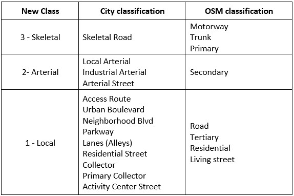
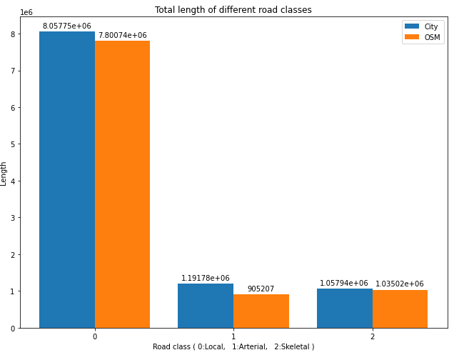
Figure 8 shows the road lengths by new classes. It can be seen that two datasets have a very close length in all three road classes. It also can be seen that the city road network has about 2 percentage more road length in all three road classes which means OSM roads have still a small proportion of incompleteness.
Positional Accuracy
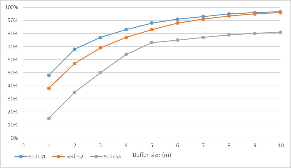
Figure 9 shows the proportions of OSM road segments that fall within the buffers of city road segments with a range from 1 to 10 meters. It can be seen that approximately all classes of roads have a logarithmic increase in their positional accuracy. The average positional offset is 2.3 meters. At a buffer size of 1 meter, the positional accuracy ranges from 14 to 49%. The accuracy increases at a relatively fast rate until 6 meters. After that, the accuracy increases very gradually. Over 86% of road segments have positional errors within 5 meters. At a buffer size of 10 m, classes 1 and 2 have over 90% of positional accuracy, and class 3 shows around 80%. However, the lengths of roads in these two classes are relatively short, which means their results may not be as representative.
Conclusion
The overall aim of this work was to evaluate the quality and reliability of the OSM road map in the city of Calgary. An interesting finding is that the local roads (rank 1) actually have the highest level of positional accuracy, while skeletal roads have the lowest level of accuracy. One of the reasons behind this could be participation inequality which means the accuracy of the VGI data in densely populated areas is higher than in remote areas. Hence, it is very difficult to generalize the OSM quality, and if OSM is to be considered for application to a project with higher than usual demands for map accuracy, there are some questions that should be answered first. Some of these questions could be:
- Are there better and more efficient methods to evaluate the OSM quality (e.g., data history analysis)?
- How can one improve OSM quality in general?
- What is the most efficient way to combine the OSM data with government data to benefit from all available data?