Natural Asset Mapping Project (NAMP) of Georgian Bay Biosphere Mnidoo Gamii: Testing Land Cover Classification
This work is Part 2 of an ongoing project conducted in collaboration with the Georgian Bay Mnidoo Gamii Biosphere (GBB) alongside Dr. Brandon Van Huizen and Dr. Chantel Markle of University of Waterloo and my supervisor Dr. Mike Waddington. This portion and Part 1 on data gap analysis was presented on GIS Day at McMaster University on November 21, 2024.
Background
In Part 1, we compiled geospatial datasets for the Eastern Georgian Bay region and conducted a gap analysis to gauge data availability. For this objective, we used some of the primary datasets we collected towards testing habitat mapping, or land cover classification approaches.
Broadly speaking, land cover classification uses remotely sensed data to create derived, thematic data of land cover categories. This can be done by manually delineating features but for all but the smallest areas this is achieved by different methods or algorithms. Methods can be unsupervised, where simply the classes are derived from the data itself and supervised, where a classification scheme is prescribed. Since we have various partners looking for specific degrees of detail (categories), we opted for the supervised approach for two prospective classification schemes. Due to the area of the entire GBB study area exceeding 7,500 km2, we took the approach of starting with a small test area before having to contend with the greater processing and memory demands of the whole study area.
Study Area
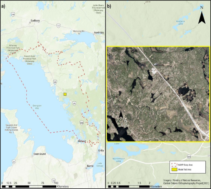
We selected an area of about 20 km2, known as the Dinner Lake area due to having been studied by the Mac Ecohydrology Lab for about the last decade and being fairly representative of the Boreal Shield landscape of Eastern Georgian Bay featuring rock barrens, wetlands, forests and ponds (Figure 1).

Classification Methods
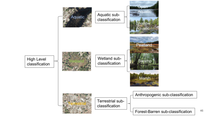
Two classification schemes were used to gauge methods’ abilities in differentiating general, dissimilar and finer land cover classes and were loosely based off of Ontario’s Ecological Land Classification (ELC) system (Table 1). Training data was created by digitizing polygons of these features using a combination of high-resolution Central Ontario Orthophotography (COOP) (Ontario Geohub, 2022) and on-the-ground knowledge of the area. The aim was to achieve similar areal coverages of each class at least at the high-level but some disparities emerged at the subclass level due to varying numbers per high-level class and low representation of swamps in the test area.
| High-level Class | Subclass |
| Wetland | Peatland (Fen/Bog) Marsh Swamp |
| Terrestrial | Anthropogenic Barren Coniferous Forest Deciduous Forest Mixed Forest |
| Aquatic | Open Aquatic Shallow Aquatic |
Predictor variables fed into the model are described in Table 2 and are derived from primary datasets; the COOP imagery (Ontario Geohub, 2022), Forest Resource Inventory lidar (Ontario Geohub, 2024a) and Ontario Hydro Network (Ontario GeoHub, 2024b), resampled to 1 m.
| Variable | Description |
| Red | Orthophotography red band |
| Green | Orthophotography green band |
| Blue | Orthophotography blue band |
| NIR | Orthophotography near-infrared band |
| NDVI | Normalized Difference Vegetation Index from COOP bands |
| TWI | Topographic Wetness Index from lidar DEM |
| DTW | Depth To Water index from lidar DEM and Ontario Hydro Network water bodies |
| Curvature | Degree of concavity/convexity computed from lidar DEM |
| NDWI | Normalized Difference Water Index from COOP bands |
| Stochastic_depressions | Stochastic depressions using lidar DEM input and Whitebox algorithm |
| CHM | Canopy Height Model from FRI lidar |
| NDVI_SD | Standard deviation of NDVI in 20m neighbourhood |
| NDWI_SD | Standard deviation of NDWI in 20m neighbourhood |
| Aspect | Direction of steepest slope |
| Slope | Maximum rate of change in elevation |
| TPI_200m | Topographic Position Index from 200m neighbourhood |
| Pit_fill | Measure of topographic roughness |
| SD_curvature | Measure of topographic roughness |
| SD_slope | Measure of topographic roughness |
| SD_residual_topo | Measure of topographic roughness |
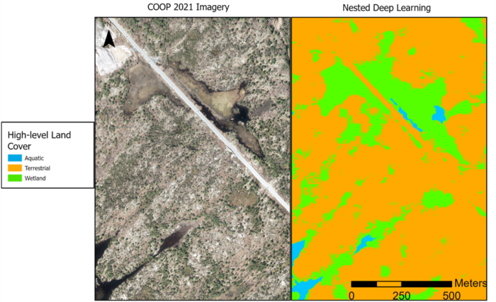
The two methods tested differed in overall approach and classification model. The first was a nested deep learning model that applied a deep learning algorithm (U-Net) through the Train Deep Learning Model tool in ArcGIS Pro 3.4 first at the high-level and then again on just the aquatic, wetland and terrestrial pixels to discern their subclasses (Figure 2). This was trained using the first 8-10 predictor variables (Table 2) to avoid excessive dimensionality.

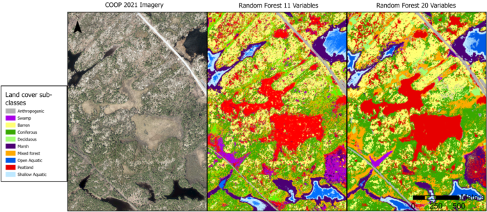
The second method was a more direct application of the random forest algorithm via the Forest-based and Boosted Classification and Regression tool in ArcGIS Pro 3.4, independently at the high-level and subclass level. These models were trained on up to 20 predictors (Table 2) in order to leverage the random forest classifier’s ability to identify variable importance. That is, how effective predictors were at differentiating land cover classes.
Accuracy Assessment
The accuracy metrics used to evaluate classifications were precision, recall and F1 using 10% of the training held back for validation. Precision is a measure of the proportion of correctly predicted pixels over the sum of correct and incorrectly predicted pixels. Recall is the proportion of correctly predicted pixels over all the pixels of that land cover type. F1 is a measure of overall model performance that averages precision and recall. To address the dependency of subclass classification accuracy on the initial high-level, accuracy metrics were computed as the product of the two. Accuracy was considered high if >0.8, moderate if 0.6-0.8 and low if <0.6.
Classification Results
At the high-level, the nested deep learning model had high recall but low precision and F1 (Figure 3). With the random forest model, recall was also high and precision and F1 improved to high as well. All were so high (close to 1) that the addition of further predictor variables had minimal effect, though it identified vegetation (CHM), topographic position (TPI) and hydrology (DTW) as the most important variables.

At the sub-class level, the nested deep learning model achieved high recall overall, again along with low precision and F1, but the specific land cover classes of mixed and deciduous forest were only at moderate recall. With the random forest classifier, the addition of the CHM as a predictor was able to achieve high accuracies across all metrics, but again with mixed forest at moderate accuracy (Figure 4). With the expansion to 20 predictors, we were able to get high accuracies across the board.

Discussion and Next Steps
While the nested approach had the benefit of making each classification operation less complex and demanding due to having to differentiate between fewer classes at a time, it had the distinct disadvantage of cascading errors that we had to explicitly take into account and potential to greatly increase processing requirements down the line as it would require more than twice as many models to be trained in total. The early difficulties with the mixed forest class, which intuitively shares similarities with the coniferous and deciduous classes, should be heeded as a warning with regards to our updated classification scheme. After discussion with partners, there is a need for outputs that align more closely with those of the Ontario ELC, which in initial conceptualization has our most detailed land cover scheme up to 25 classes. This will also come with greater requirements for ground truthing to support training data for habitat mapping as, for example, the peatland subclass in this test example would be broken down into bog and fen, as well as the open, shrub and treed variants thereof.
To foster greater accessibility and transparency among partners, we are currently shifting towards an open source approach in R. This offers a few other benefits, including the ability to more easily intercompare classification approaches trained in the one script and the potential to leverage cloud computing that might be necessary to speed up or make the task feasible for the entire GBB study area. Memory requirements will become a concern as the 20 predictor variables at 1 m resolution exceeded 1 GB in size for this test area that was less than 0.3% of the size of the broader study area. This can be alleviated by further optimizing our predictor set using the random forest’s variable importance, but this will end up well exceeding the RAM capacity of any regular desktop.
While we stuck to pixel-based classifications of the deep and machine learning varieties here, we observed visually that there was a tendency to produce ‘noisy’ outputs. This may reflect reality given the mosaic landscape of the Boreal Shield along Georgian Bay but cleaner delineations may have greater utility from a planning or land management perspective. It’s for this reason we will be exploring image segmentation as part of our next steps in testing.
References
Ontario GeoHub (2022). Central Ontario Orthophotography Project (COOP) 2021 – 1km Index. https://geohub.lio.gov.on.ca/datasets/lio::central-ontario-orthophotography-project-coop-2021-1km-index/about
Ontario GeoHub (2024a). Ontario Forest Resources Inventory. https://geohub.lio.gov.on.ca/pages/forest-resources-inventory
Ontario GeoHub (2024b) Ontario Hydro Network (OHN) – Watercourse. https://geohub.lio.gov.on.ca/datasets/mnrf::ontario-hydro-network-ohn-watercourse/about
R Core Team (2024). R: A language and environment for statistical computing. R Foundation for Statistical Computing, Vienna, Austria. URL https://www.R-project.org/
