
Assessing Carer-Worker Potential Path Areas with Python and ArcGIS Pro
I’m so excited to be commencing my graduate studies back at McMaster, working in the School of Earth, Environment & Society’s Transportation Research Lab (TransLAB) — where I have the opportunity to pursue interesting research projects about transportation and travel behaviour problems, with GIS.
In my last term of undergrad and through this past summer, I’ve had the opportunity to work with my Master’s Supervisor Dr. Darren Scott, Dr. Allison Williams, as well as several other colleagues from McMaster and Simon Fraser University, on a project to assess space-time constraints on Carer-Workers in the Greater Toronto-Hamilton Area. We did this through the use of Potential Path Areas, and ArcGIS Pro was invaluable throughout the process.
Who are Carer-Workers?
Carer-Workers are a segment of the population who are formally employed, while also providing informal, unpaid care to an adult recipient (such as an elderly parent or an adult dependent child). Carer-Workers are likely to have significant space and time constraints on their lives, due to the dual responsibilities of employment and those for whom they are providing care. Carer-Workers are estimated to be more than a third of Canada’s workforce!
What is a Potential Path Area?
I’m glad you asked! Potential Path Areas (PPAs) are a piece of a Space-Time Prism — an important measure of space-time accessibility based on crucial time-geography work by Hägerstrand in 1970. While a Space-Time Prism captures time as an additional dimension, PPAs focus on the “space” component. In essence, a PPA is the total area, or total length of paths (roads) available to an individual, between an Origin and a Destination, within a particular time budget.
Let’s say, for example, that a Carer-Worker works until 3:00 PM on a weekday. At 4:30 PM they must go to a doctor’s appointment with their elderly parent, for whom they care regularly. Their work is the Origin; the doctor’s office is the Destination. Their Travel Time Budget (TTB) is 90 minutes. A PPA is the total area or length of roads this Carer-Worker can access in this 90 minute span, for any length of time, while still making it to that doctor’s office with their parent on time. These PPAs must be between fixed activities — those being activities with rigid scheduling and mandatory participation, such as an appointment or work. Many activities, like shopping, are considered flexible as they can take place at any time.
The Analysis:
Using Travel Diaries for 15 Carer-Workers in the Greater Toronto and Hamilton Area, we constructed daily aggregated PPAs for each study participant, to compare sizes — and therefore, accessibility — across a range of demographic indicators. For example, we may want to be able to determine if female Carer-Workers more space-time constrained than their male counterparts, or whether those in higher-earning households less constrained than those in lower income households. Travel Diaries were deconstructed into fixed activities, to make the start and end points for PPAs. Then, we generated the PPAs using these start and end points. We did this through several methods. Tying them all together was done easily using ArcGIS Pro and ArcPy .
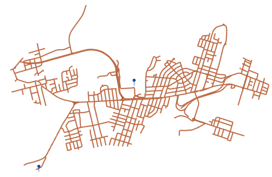
For those PPAs between a point A and point B (that is, the start and end points were different places), we developed a custom PPA generation script in Python (using the OSMnx Python Module) to generate a polyline shapefile of the PPA, given an origin coordinate (Latitude/Longitude), destination coordinate, and a travel time budget in seconds. The OSMnx Module used the OpenStreetMaps Road Network data to generate the estimated PPA. The image above is an example output from this Python script.
For PPAs with the same start and end point (leaving work to come back to work a little later, e.g.), we used two of ArcGIS’s Service Area tools. For those trips under 15 minutes, we used the Ready-to-Use Generate Service Areas Tool in ArcGIS Pro and ESRI’s Online Road Network Dataset. Trips greater than 15 minutes in length were generated using the Service Area Network Analyst Tools in ArcGIS Pro, and a Network Dataset for all of Canada from DMTI Spatial.
Aggregating Different PPAs:
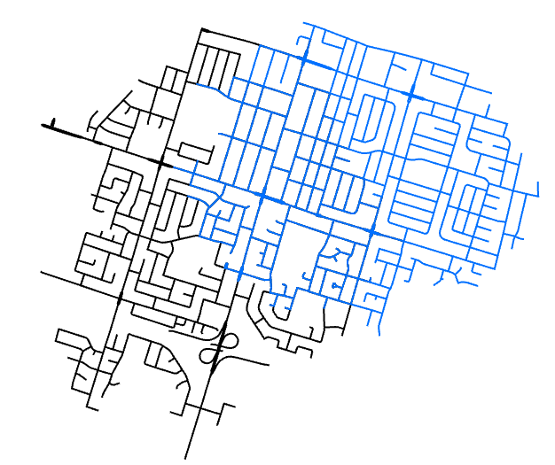
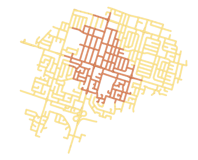
What we really wanted was to aggregate these individual trip PPAs into one participant’s daily PPA — all the places they could get to, given the space and time constraints of their day. However, this was quite challenging, because we had PPAs generated from 3 Network Datasets, and each one was slightly different from the other. ModelBuilder was perfect for creating a method to aggregate them and testing it.

Despite this model’s simplicity, it was very effective in merging the different PPAs. It converted the line shapefiles into polygons, via a buffer. It then merged the buffers into one shapefile, and Dissolved them to remove any overlaps of the polygons. Finally, it was converted back into lines using the Polygon to Centerline tool, which approximated the actual road lengths.
This method was greatly improved by using ArcPy to automate the process, because several days had many PPAs to be aggregated, and this is a repetitive task that is both easier and quicker to implement through scripting. Using Python, I could quickly generate daily PPAs and get to analyzing the data!
# PPA Aggregation Process
import arcpy as ap

# Setting Workspace
ws = ap.env.workspace = "C:/exampleDirectory"

# Get each day's individual PPAs (Contained in "C:/exampleDirectory")
FCs = ap.ListFeatureClasses()

# Using a loop, iterate through the PPAs, creating buffers and giving them a distinguishable name
for features in FCs:
	descFC = ap.Describe(features)
	ap.Buffer_analysis(features, "C:/FileStorageSpace/" + descFC.baseName + "_BUFF", "5 METERS", dissolve_option="ALL")

# List the Buffer FCs, and Merge them using Union
ws2 = ap.env.workspace = "C:/FileStorageSpace"
buff = ap.ListFeatureClasses()

unionFC = ap.Union_analysis(buff, ws2 + "/PPA_Union")

# Dissolve all buffers into one large daily PPA buffer
dissolveFC = ap.Dissolve_management(unionFC, ws2 + "/PPA_Dissolve")

# Create final PPA by estimating the Centerline of the daily PPA buffer
ap.PolygonToCenterline_topographic(dissolveFC, ws2 + "/DailyPPA_1")
Comparison of these PPAs was done by projecting all PPAs into NAD 1983 UTM Zone 17N (an accurate Projection for Toronto and Hamilton), and calculating the sum of the road lengths in the features’ geometry.
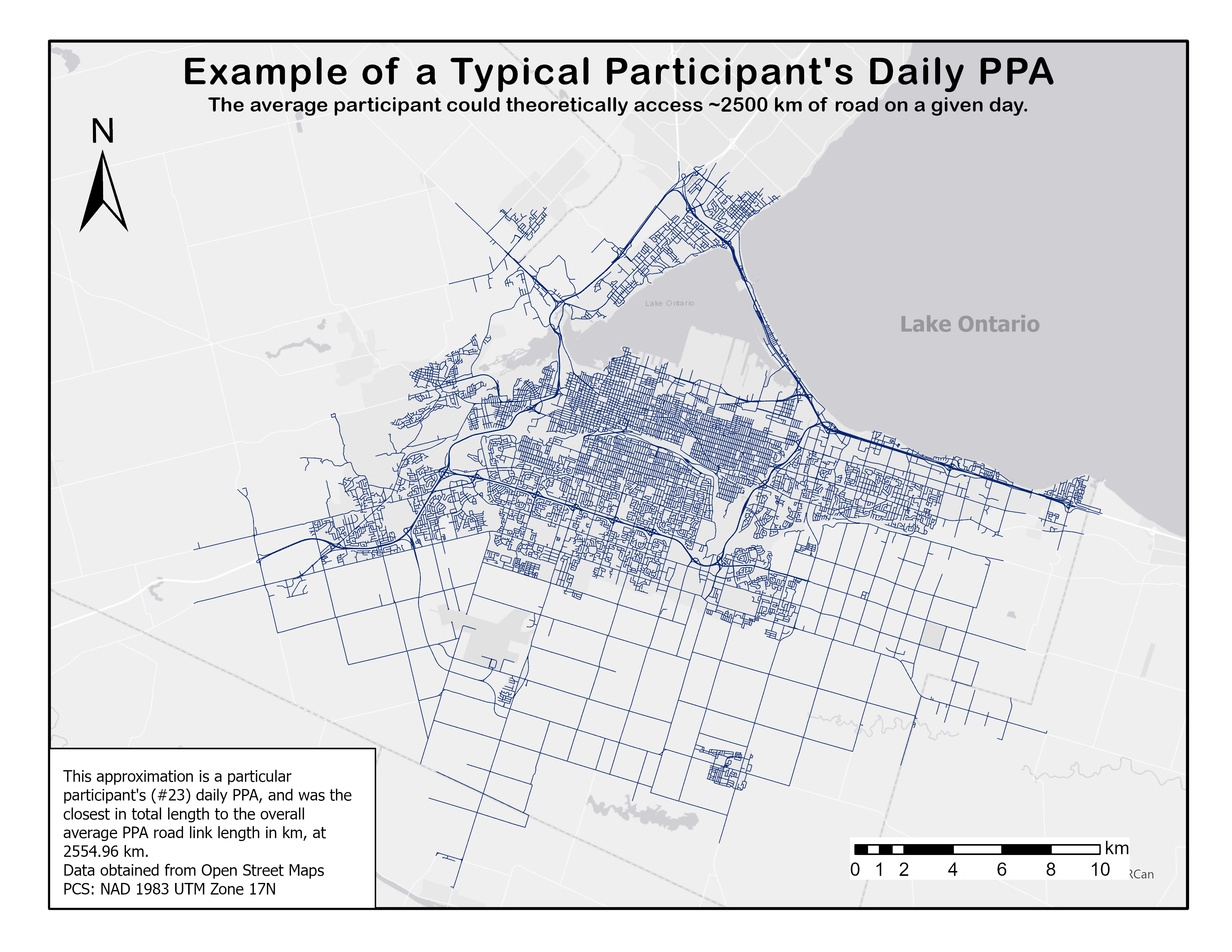
The map below is an approximation of the size (total km of road length accessible) of the average participant’s daily PPA size. The average daily cumulative road length in km for participants was 2591.15 km — meaning that, on the average day, over the course of that day, there were 2591.15 km of roads available to a participant, given their personal time constraints listed in their travel diaries. These distances are theoretical. They are what the participant could potentially access on an average day, given their time constraints.
Wrapping it all up: ModelBuilder, Network Analyst and ArcPy to the rescue!
Much of the analysis and data generation for this project would not be possible without the embedded tools in ArcGIS Pro, and the ArcPy Python module. Service Areas were essential for developing an approximation for a PPA using the same Origin and Destination point, and ArcPy made aggregation more convenient, reproducible and streamlined. While the analysis for the project is still ongoing, I am so thrilled to have been part of such an interesting, challenging and multi-faceted project, and ArcGIS has been crucial to its success.