
GIS Summary of SNAP 2019 (Part 4): Multi-Criteria Data Analysis
This is the last article in the 4-part series summarizing work completed by Todd Wong for the Stelida Naxos Archaeological Project (SNAP). For more background and steps leading up to the analysis presented in this article, refer to Part 1, Part 2, and Part 3.
Introduction
Multicriteria Data Analysis (MCDA) is a collection of formal approaches which seek to take explicit account of key factors or variables in helping individuals or groups explore decisions that matter and has been involved in the spatial analysis industry (Greene et al. 2011). This form of data analysis involves the combination of layers with relative weights. Weights are decided in multiple ways, in our case we will be using what is referred to as Analytical Hierarchy Process (Greene et al. 2011). The analytical hierarchy process involves the use of ranking methods and pairwise comparison matrixes to formulate weights that will be applied to each layer (Jankowski 1995). For our methods, I will be using a method similar to ideal point, which is an identified point within the criterion that will be used for the analysis, in which we take the averages or modes and apply fuzzy memberships or linear standardizing methods to produce weighted layers (Greene et al. 2011).
Analytical Hierarchy Process
These weights/scores are interpreted as percentages from 0 to 1, with higher percentages being the most important. When adding up all the elements that make up the Analytical Hierarchy Process (AHP), the sum of all the weights is 1, representing the highest score possible in the final result. In our case I performed AHP in two levels. The first level is a categorized level that will be broken down into another AHP in the second level. For instance, the Distance from Waterbodies category is broken down further into rivers, coastline, and springs. In this case the layers will be given ideal points where the point within the criterion is scored the highest and values away from this point are gradually scored lower as they move away from this ideal point.
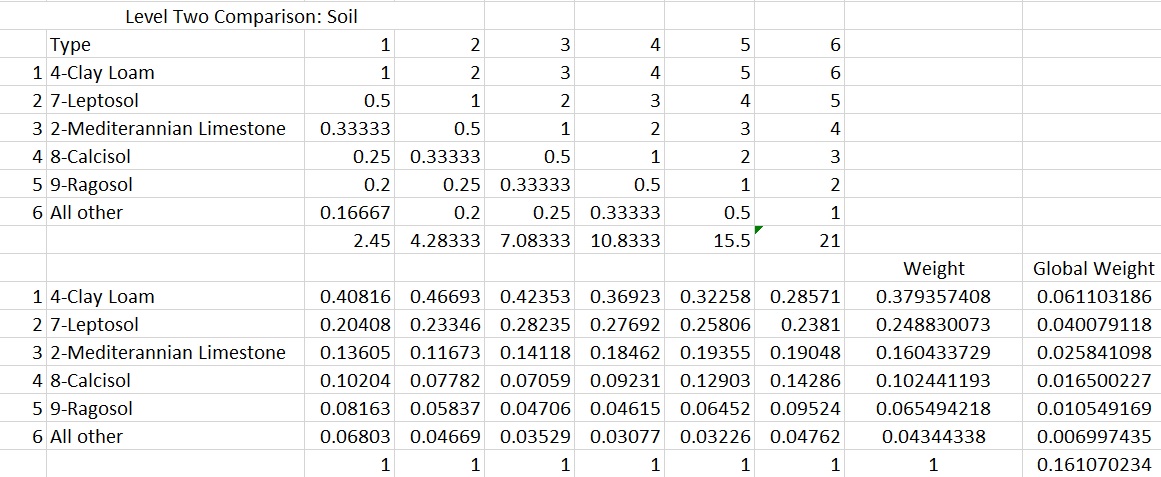
The first level can also be one layer that is classified or discrete such as the Soil and Lithology layers. In discrete layers there are different types and each type has more importance over the other. In order to establish which types are the most important and which are the least, a pivot table is created from the All Landscape Statistics workflow to establish a count of each of the majority types at each site. From here you order each one by taking the type with the most counts and ranking it the highest and then going down to the second most and so on, with the last ranking being “Other Types”, which are the types that were not included in the pivot table.
Thematic Layers: Surface Morphology
Elevation
The elevation layer was derived from the ASTER GDEM sensor that produces a 30 meter by 30-meter resolution raster layer. The mountainous island ranges from 0 meters to 990 meters above sea level. According to our Excel analysis the sites are typically found at around 233 meters in elevation. For this raster layer we used a fuzzy Gaussian membership with a spread of 0.00005 in order to create larger scores away from this singular elevation which was set as the midpoint of 233 meters. This creates a score layer in which the highest score is 233 meters with scores getting lower as elevations get lower and higher from this elevation.
Slope
The slope layer was produced from the previous elevation layer using the Slope tool with a planar method. The slope ranges from 0 to 60.6645. Based on the results from the various workflows that I produced, the sites tend to have lower slopes, meaning that the sites on the island favour gradual slopes on the island. Similarly, to the previous layer the fuzzy Gaussian membership was used with a spread of 0.005 and a midpoint of 11.2053 applied, scoring the higher slopes much lower and the flat areas higher. In general, the slopes appear to favour the lower slopes, meaning that the flatter terrains will be of higher scores as we wanted.
Thematic Layers: Distance from Waterbodies
Distance from Waterbodies were ranked by their average distance from waterbody features. This means that the feature with the smallest average was ranked the best and the one with the farthest was ranked the least important. The rank is as follows: (1) Rivers, (2) Coastline, (3) Springs. For each of these a Maximum Score Procedure was applied to standardize the layers from 0 to 1.
Distance from Rivers
River features were created from digitizing rivers using a topographic map created by Penelope Matsouka. The distance away from these features was determined by averaging the distance from the rivers to sites created by the Near Statistics workflow. The average distance from rivers to sites is 504.619 meters, and this value will be used for our ideal point. In order to achieve this a buffer was created from the river with the dissolve option checked in order to create a singular feature rather than multiple buffers that would distort our results, with the ideal point being the distance parameter. The buffer was then converted to a line and clipped to the study area; as some buffer extended outside of it. The Euclidean Distance tool was than performed, with the input source feature being the lines that were created. The layer was then standardized using a linear cost method, which allows for the closer values to be scored higher with a rank between 0 to 1.
Distance from Coastline
The coastline was derived from a boundary file of Naxos and traced in order to create a singular line. As before, the near statistics workflow was used to find the closest distance between site and coastline. The average and ideal distance between the two features was 1523.3445 meters. This tells us that the sites are relatively close to the coastline, although we are limited to the current coastline of Naxos. For this feature buffers were also applied to the coastline and then converted to line features as I did with the previous example. The Clip tool was then applied with the original boundary polygon to keep the lines within the study area of Naxos, as the Buffer tool created polygons that extend past the study area. The Euclidean Distance Tool was then used as it was with the river distance and then standardized the same way.
Distance from Springs
Spring locations were digitized into the GIS environment the same as the river shape files were, using a topographic map created by Penelope Matsouka. The near statistic workflow produced an average of 3286.9221 meters away. This large number is due to the lack of sites found in the northern region of the island, where most of the springs reside. The same methods as the previous two variables were used to create the ideal point rasters.
Thematic Layers: Classified/Discrete Variables
Soil
Soil was chosen over lithology because of its importance for the development of crops on the island, with the previous two categories of thematic layers allowing this cultivation to be possible. The soil layer was created using several soil maps from different datasets that were georeferenced into the GIS environment with both coarse and detailed resolution. Detailed maps were only found for the southern region, while the coarser maps were in the north and used to fill holes in the remaining map. The limitation of this is sites found in these coarse regions only have one soil type. To standardize these layers the weights (%) that were established using the Analytical Hierarchy Process were then multiplied to generate a score. The top-ranking type that was established in the pivot table has the highest rank, while the category of “Other Types” would have the lowest. Using the Reclassify tool, we changed the value of the original layer to create a score layer which is then converted to a float raster, which has the ability to be divided into decimals, unlike the reclassified layer. The score layer is then divided by the number it was multiplied by in the Analytical Hierarchy Process in the Raster Calculator tool to become the standardized layer.
Lithology
Surface lithology was established from a detailed map produced by the National Institute of Geological and Mineral Research that was georeferenced into ArcMap. The same method for the soil involving the All Landscape Statistics workflow and Excel were applied to discern ranks among the lithology types. The standardized layer was created in the same manner that the soil was with the reclass, float, and raster calculator tools.
Results
To obtain the final result, the Raster Calculator was used to add all the layers together. To make this process easier, the layers in the first two categories (first level AHP) were multiplied by their global weight to produce rasters with the proper weights and scores. As mentioned in the previous section, classified/discrete were standardized in a way so that each type was given its own global weight using multiple tools to transform the data into the weighted layer. All layers were then added together in the Raster Calculator to produce the result raster that possess a score from 0 to 1, with 0 being the lowest and 1 the highest. The raster was then classified into 5 categories; (1) Very Poor: 0-0.2 (2) Poor: 0.2-0.4 (3) Moderate: 0.4-0.6 (4) Good: 0.6-0.8 & (5) Very Good: 0.8-1.0 (Figure 4). Suitable areas are considered to be areas classified as Good and Very Good, which makes up just over 50% of the total area.

Conclusion
Using ArcGIS workflows such as model builder and python to create tools that were designed to extract landscape information from rasters, I was able to create and formulate rankings for the analytical hierarchy process at the second level with the help of some research at the first level to rank the categories. The resulting ranks of the AHP allowed us to create a site suitability raster, that could lead to the discovery of new sites due to the commonality of landscape that were discovered in the landscape statistic tools.
References
Greene, R., Devillers, R., Luther, J. E., & Eddy, B. G. (2011). GIS‐based multiple‐criteria decision analysis. Geography Compass, 5(6), 412-432.
Jankowski, P. (1995). Integrating geographical information systems and multiple criteria decision-making methods. International journal of geographical information systems, 9(3), 251-273.