
GIS Summary of SNAP 2019 (Part 3): Analyzing Extracted Results
This third part of my four-part series will go through a case study in which we analyze and determine variables generated from several tools. Our case study involves 50 early bronze age sites on Naxos (Figure 1), an island located in the Aegean that is the largest of the Cycladic sister islands with a rich archaeological history. We will be analyzing several statistical types that are important in both the individual site analysis that were generated using the tools and workflows that I created in my previous post, as well as discussing these important statistical types used in our analysis. Through each statistic type we will look at an example of where these come into play in our case study on Naxos, while also developing a quantified settlement pattern.

Statistical Manipulation: Averages
Averages are important for both the file layers and the statistics that were generated for these files. Average statistics should be considered when analyzing variables such as elevation, slope, and curvature. These statistics become knowledge in a variety of ways. For instance, with slope we want to know if the area has more steep or gradual slopes and by using mean we can get a general idea of whether the area leans more towards one or the other. With elevation, it is important to consider the general elevation of sites; that might be linked to certain views or viewsheds of the area, which is best determined using mean or median. In order to determine averages and ideal values for multi criteria analysis, the Summary Statistics tool was used and results recorded in an Excel sheet to keep track of ideal values.
Statistical Manipulation: Mode & Majority
Mode statistics as generally done for discrete raster files, such as soil, lithology and land class. In our case I looked at Soil and Lithology for modal analysis. The outcome of the statistic tools shows the most common feature type within the immediate area of each site. This analysis tells us what the favored type is for each site, and this is when exporting the results to Excel becomes more user friendly for archaeologists. In Excel, you will take the column and create a pivot table that counts the number of modes for each type in the raster to formulate which discrete feature type (i.e., Soil type) is favored in our study areas. In our case, this can assist with multi criteria data analysis through the ranking of types based on the number of counted modes.
Statistical Manipulation: Correlations
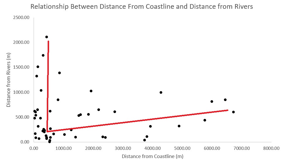
The next thing that can be looked at is correlations in site location regarding certain features. This was mostly done for the different water body features that were being analyzed in our case study. For instance, one of the items I looked at was the distance between rivers and coastlines. I took the distance from these features using the near statistics workflow we created, and compared them in an exported Excel file that was generated from the table to Excel script in ArcGIS Pro. Excel was chosen because not all archaeologist might have access or practical knowledge of the integrated table and graph functions in ArcGIS Pro. The graph shows us an L pattern in which we can discern that the sites are either close to the river or coastlines but not both for half the locations, while there is a cluster near the origin (Figure 2). This can tell us about water feature preferences in choosing site locations for cemeteries and settlements.
Naxos Case Study: Deriving Settlement Patterns from Landscape Statistics
The table below (Figure 3), displays the statistics derived from the tools that were created for this analysis. For the All Landscape Statistic workflow, the immediate area/radius was set to 500 meters. These results that were attached to the original site file through the use of the tools created in the last blog that allowed us to export the table to Excel without any further shuffling of data once it was in Excel. The first two columns are average statistics of the surrounding elevation and slopes, telling us what the typical elevations in the area were and if the area has a series of gradual or steep slopes. The next three used the Near Statistics workflow to derive distances from several waterbodies; river, coastlines, and springs. The final two columns are lithology and soil type which are displayed as numbers that represent coded values for each type.
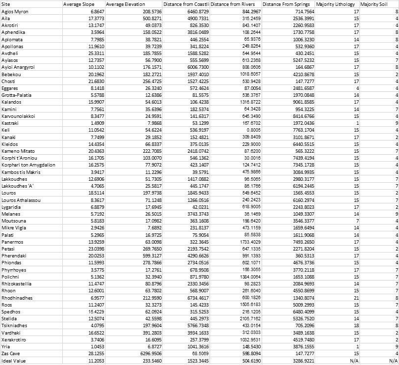
In order to derive settlement patterns, we must manipulate the data using statistics and pivot tables. For the first five columns the average of the entire column was deemed to be the desired statistics type because that will give us an idea of where most of these sites are found. For the remaining two columns a pivot table in excel was created to count the number of each type to find out which was the most common and least common for all sites (Figure 4).
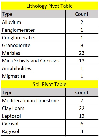
Using these methods, we are able to give quantified results for settlement patterns rather then generalizing them. From this we are able to determine that sites are typically found around areas with an elevation of 233 meters with slopes around 11 degrees. There are several water sources that could have been used in the area. Rivers are the closest of the water features from all sites with the average distance being around half a kilometer away. Springs are the farthest water feature at an average of 3.28 kilometers away from sites; which is due to the fact that most of the springs are located in the north while a majority of the sites are located in the south. Sites are typically around a kilometer and a half from the coastline, putting them relatively close to the Aegean Sea. For the soil samples the most common type is Clay Loam with the second being Leptosol. For surface lithology we found that the most common type are Marbles, while the second is Mica Schist.
The statistics of each site and their resulting commonalities and averages can tell us a lot about the surrounding area around sites in our case study. The commonalities are then transformed into settlement patterns with quantified results. With these results we will now be able to perform a multi criteria data analysis with these values to come up with a map that shows possible site locations that have yet to be discovered. In order to achieve this, several techniques performed in a GIS environment were used to create what are known as ideal points, a method of multi criteria data analysis that will be utilized in the next blog post.