Data Wrangling with Python and R, Part 1: “Fun” with LiDAR Buffers
One realization that keeps hitting me throughout my MSc is how many little things need to be dealt with in order to do even basic analysis using real-world data. My supervisor once told me that about 70% of the work that gets done in our lab is what he calls “data wrangling”, which I would now agree with any day of the week. In this post, I’ll be giving an example of a seemingly small issue with some LiDAR I’m working with that required a much more complicated fix than it first appeared.
1) Identifying the problem
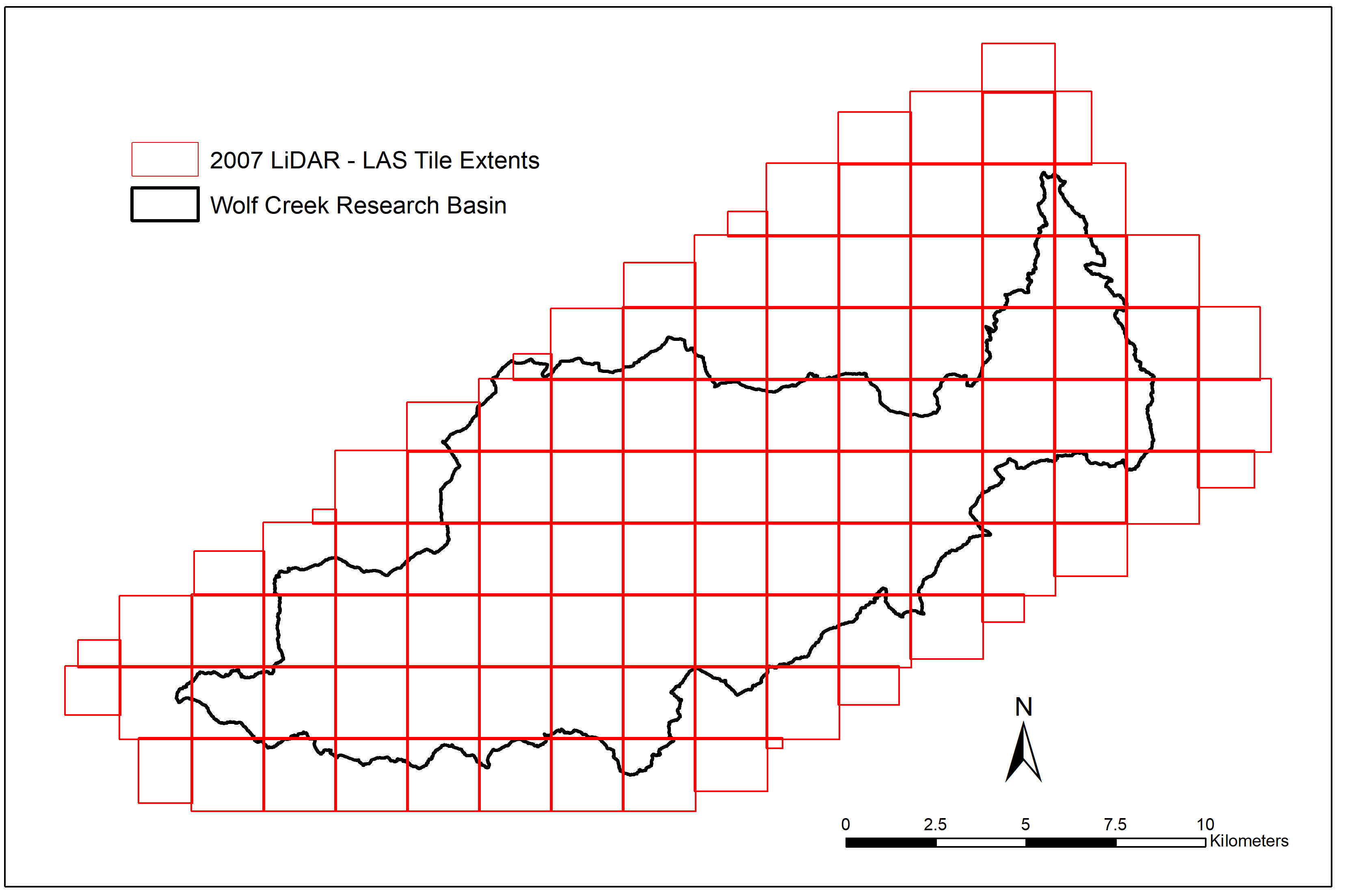
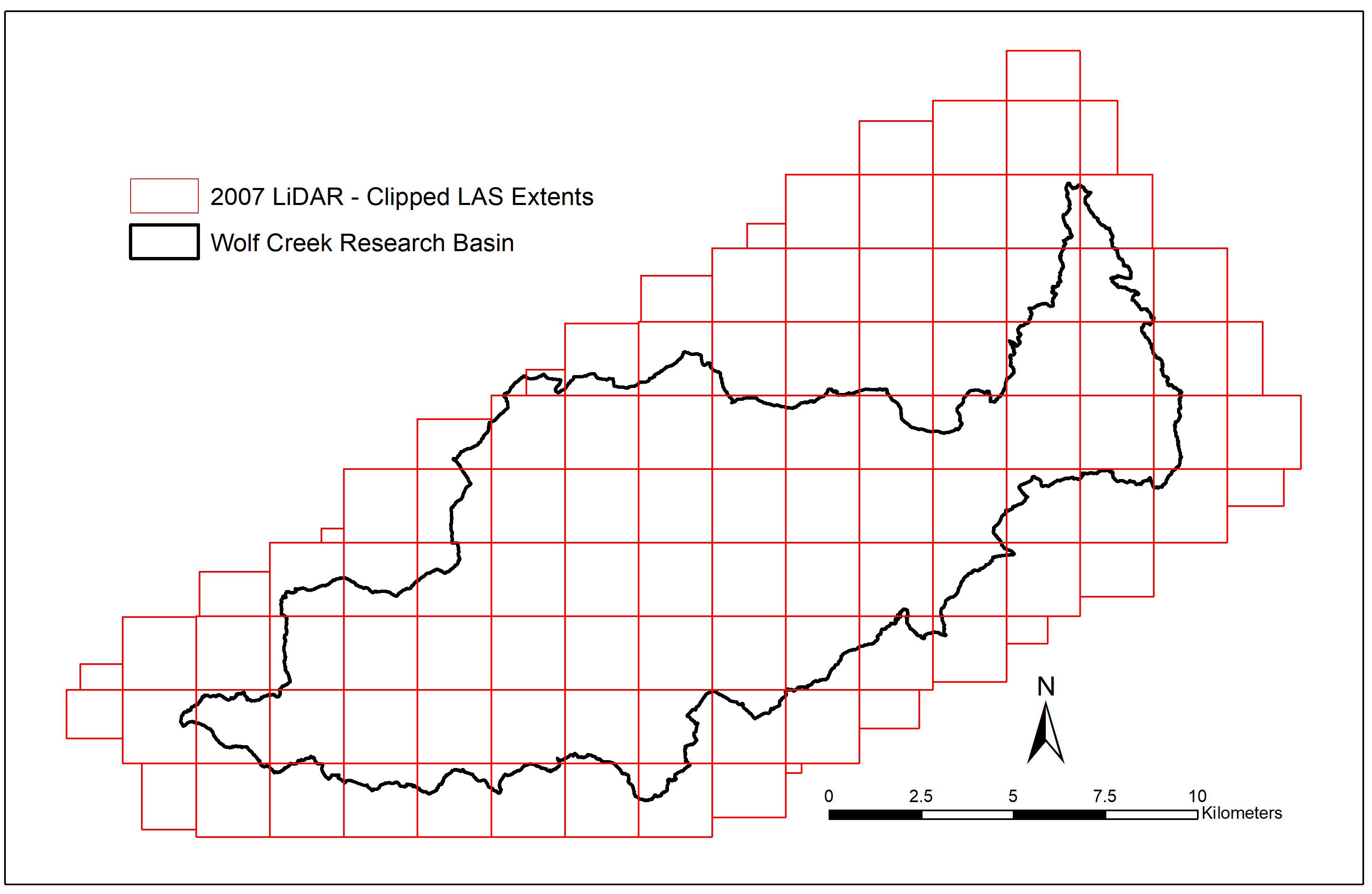
As anyone who’s read my previous posts might know, my research focuses on using multi-temporal LiDAR and optical imagery to evaluate vegetation change in the Wolf Creek Research Basin from 2007 to 2018. The 2007 LiDAR survey we’re using for this was delivered as 115 separate tiles in the ASPRS .las file format, each measuring 2km by 2km with 20m buffers on either side. As seen in this blog post from Martin Isenburg (creator and CEO of the LAStools LiDAR processing software), the creation and use of buffers when working with tiled LiDAR is absolutely necessary to avoid unwanted edge effects.
However, as the pre-processing of this data was done back in 2007 with the TerraScan and TerraMatch software packages, these buffered points weren’t explicitly flagged in such a way the software I’ve been using could read. If the point cloud was tiled using LAStools (which I primarily use when working with LiDAR), I could add additional command-line options when running lastile (such as -flag_as_witheld) to make sure that the software knows which points are buffers and which are original tile extents. Once buffers are explicitly identified, it’s easy to throw in an additional argument in future calls to LAStools (-ignore_witheld or -use_tile_bb) to make sure they’re ignored when necessary.
2) Exploring options
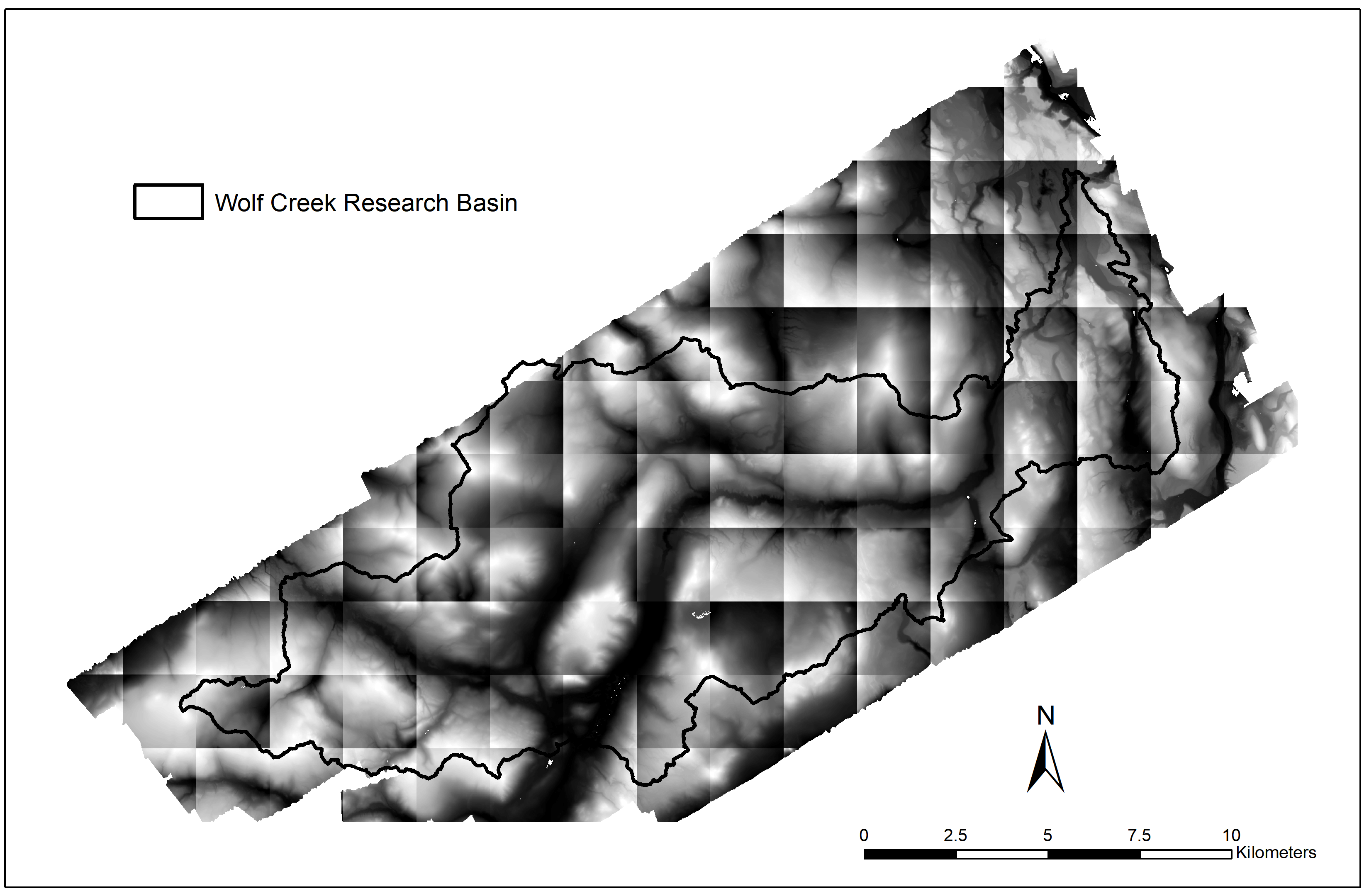
The obvious solution for this would be to use lasduplicate to identify and remove returns with identical XYZ coordinates, but as we hadn’t yet purchased the fully-licensed version of LAStools there were small amounts of noise introduced for each point so they didn’t match up. I knew that for this fix I’d need to create polygons for the original extents of each LAS tile and then clip each one of them to their corresponding extent through a FOR loop. I also remembered that each LAS tile provided had an ASCII DEM along with it, with the same file IDs as each tile. At first I thought I’d be able to just convert the DEMs to polygons, dissolve each one, then use them as clip polygons, but found out after a bit of exploring that these included the 20m buffers as well. Even with this original plan not working out, these DEMs would turn out to be very helpful in an unexpected way.
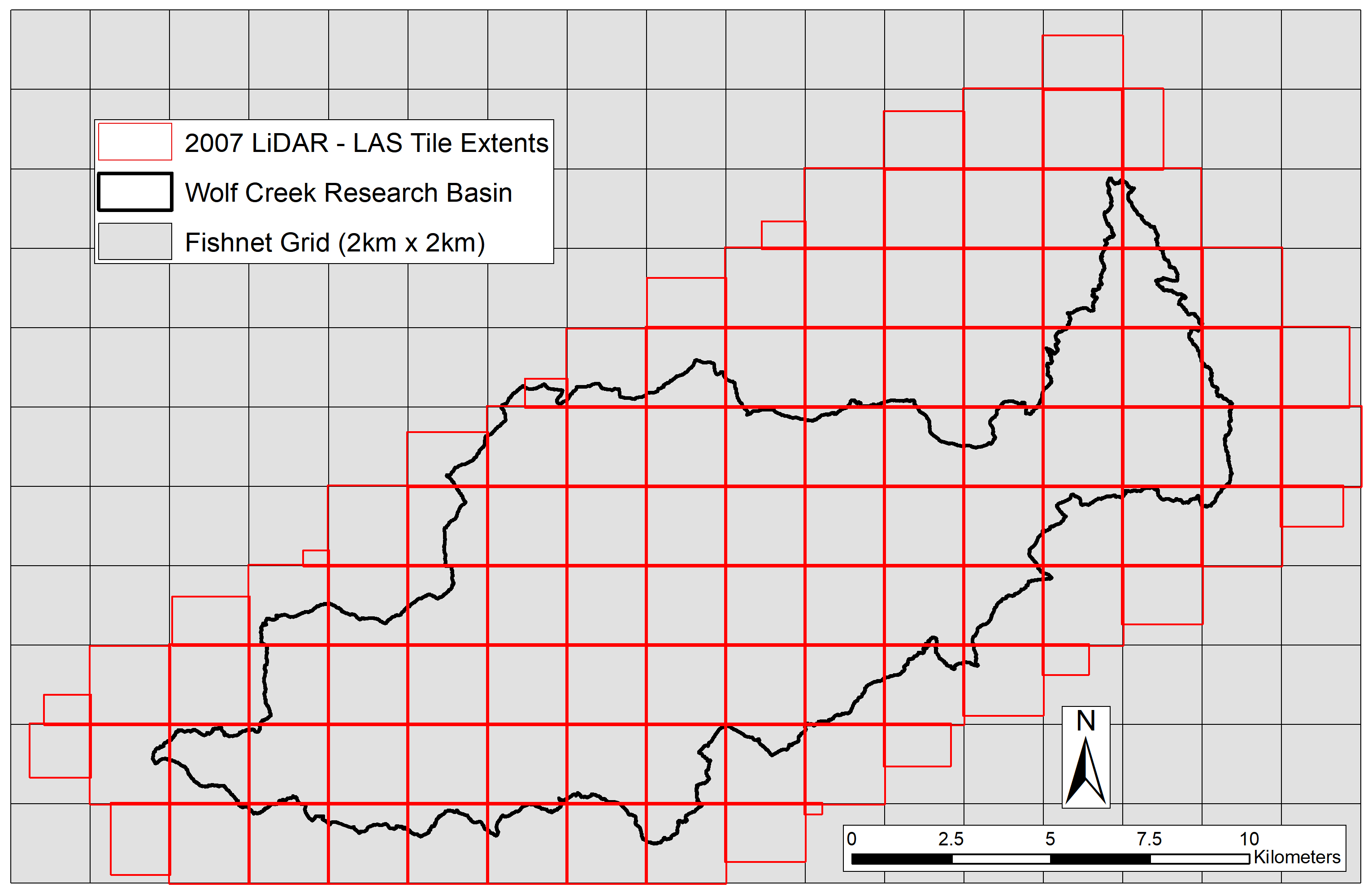
My next idea was to manually create a new grid with tile extents in ArcGIS to use as my clip polygons. Knowing that each tile measured 2km by 2km, it would be easy to create a fishnet grid with 2km by 2km cells starting on the origin of the 1st tile. This was a good start, but I’d need to find the exact coordinates to start the fishnet and a way to tag LAS tile names to their corresponding fishnet grid tiles. Though the LAS tiles only had their unique identifiers in the file names, (e.g., wolf_002_all_pts.las), each DEM tile was named using the tile ID and UTM coordinates for its north-west corner (e.g., wolf_002_G_5005_67215.asc). Using this information, I was able to create a fishnet grid with full coverage of the LiDAR extent as the first step to my solution.
3) Implementing the solution
The final fix to this problem involved 3 stand-alone ArcPy scripts, some manual editing, and one R script. I’ll go over each part of this solution and show a bit of sample code for each script used.
Once the fishnet grid was created using corner coordinates of the most south-east LAS extent, each “cell” in the fishnet still needed to be tagged with its corresponding LiDAR tile ID. Fishnet cells that didn’t overlap with any LAS tile also needed to be removed. This is where the 1st ArcPy script and the DEM tiles came into play. As they (mostly) overlapped with the fishnet grid and contained each tile ID within their file names, I knew they could help me here. I realized that if I vectorized each DEM then intersected the centroid of that polygon with its corresponding tile from the fishnet grid, I could tag each grid “cell” with its tile name. First though, I had to use a FOR loop to project the rasters and convert all the cell values to integers with a value of 0 to simplify the vectorized outputs.
#Use Spatial Analyst operators to convert all values to 0 (for cleaner polygon conversion)
for raster in rasList:
    print(raster[:-4])
    #Rasters are unprojected, so use Define Projecton (WGS84) to match 2018 dataset
    arcpy.DefineProjection_management(raster, arcpy.SpatialReference(32608))

    #Need to use Raster() function here to convert from string to raster object
    #Need to use Int() in order to convert to polygon in next loop
    outRas = Int(Raster(raster) * 0)
    outRas.save(outPath + raster[:-4] + "_extent.tif")
Another loop was used after this code block to convert each new raster into a separate polygon shapefile. This gave me a folder of 115 individual shapefiles, each named according to the DEM tile of which its extent represents.
The next step here was to use the DEM tiles to add naming information to the fishnet grid tiles. Using another ArcPy script, I added a new field in each of the DEM tiles called Full_ID to store this. By slicing the name of each tile I could store that as an object and use it in the Field Calculator to populate Full_ID. Once each tile had its name stored in this field, I merged them together then created a new point shapefile with tile centroids using Feature to Point.
#Loop over list and add fields with relevant info to each shp
#1st add field, then populate, then repeat
for fc in fcList:
    #Add field to hold full tile ID (i.e. wolf_002_G_5005_67215), then use file name to populate
    arcpy.AddField_management(fc, "Full_ID", "TEXT", "", "", 21)

    #Define function to populate FULL_ID with file names in field calculator
    fc_name = '"' + str(fc)[:-11] + '/"'
    print(fc_name)
    arcpy.CalculateField_management(fc, "Full_ID", fc_name, "PYTHON")
Once the resulting points were tagged to the fishnet grid using a Spatial Join, I used Select by Location and an edit session to remove any tiles that didn’t have an overlapping DEM centroid. I then ran one last ArcPy script to deconstruct the grid into each of its individual tiles, with their file names taken from the Full_ID field created in the 2nd script. This was done by creating a list of rows in the original shapefile using a SearchCursor and a pre-defined function to export each individual row as a new shapefile with Select.
# Create list using cursor to iterate through rows in fishnet polygon
rows = arcpy.SearchCursor(fc)

# Loop through rows in polygon and create new shapefiles from each
for row in rows:
    #Create WHERE clause using field with tile ID
    Name = row.Full_ID
    whereclause =  buildWhereClause(fc,"Full_ID",Name)
    print(whereclause)

    #Create output FC with matching name to LAS tile IDs
    arcpy.Select_analysis(fc, ws + str(Name) + ".shp", whereclause)
After this script was run, I now had 115 new shapefiles with exact coverage of each original LAS extent and the same name as their corresponding tile.
For the last part of this fix, I’d have to loop through the LAS tiles and clip each of them to their corresponding extent polygon. This is definitely possible with LAStools, but I’m much more comfortable running loops in Python or R than through command-line scripting. A great resource I’ve recently discovered is the lidR package, which is designed for working with LiDAR in R. I used different functions in this library to read each LAS file into R (readLAS), clip them to the polygon extents (lasclip), and save the results to file (writeLAS).
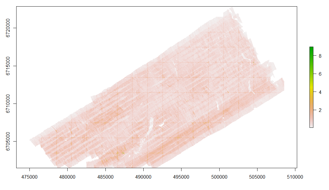
After creating lists of clip polygons and LAS files, I ran them through a FOR loop to clip each LAS by its corresponding extent tile. Since each LAS file and its corresponding extent polygon had identical base names, I could use a counter variable and indexing to make each was clipped to the proper one. Here’s what the R code for this part and the resulting clipped LAS tiles look like:
#Initialize counter variable
ct <- 1

#Create loop for clipping individual tiles
for(i in tiles){

  #Create LAS object from lasList using counter variable
  inLAS <- readLAS(lasList[ct])
  print(lasList[ct])

  #Define output file name to use when saving clipped LAS object
  #Takes base name from Full_ID field in clip tile, then appends to output folder path
  outName <- paste(tiles[[ct]]@data$Full_ID, ".las", sep = "")
  outFile <- paste(outPath,outName, sep = "")
  print(outFile)

  #Clip each LAS object to corresponding tile extent, then save new LAS object to file
  outLAS <- lasclip(inLAS, tiles[[ct]])
  writeLAS(outLAS,outFile)

  #Increment counter variable
  ct <- ct+1
}
Hopefully this helps introduce some of the struggles when working with real-world data and how many different tools you might need in your toolbox to properly handle them. In my next post, I’ll be talking about some more data wrangling from my LiDAR validation campaign this past summer involving post-corrections for differential GPS survey data.

