
Random Forest Classification with R and Collector for ArcGIS
I’m currently in my 1st year of my M.Sc degree at McMaster University, working in the Watershed Hydrology Group under Dr. Sean Carey. My research focuses on evaluating vegetation change in Wolf Creek, Yukon Territory through fusion of remotely sensed data.
My main objective is to use a combination of LiDAR (Light Detection and Ranging), optical imagery, and field methods to measure temporal changes in vegetation properties over the well-studied Wolf Creek Research Basin (WCRB). Here I’ll be talking about the landscape classification portion of my work, and how a couple of recently updated pieces of software will be making my life easier in the lab and in the field.
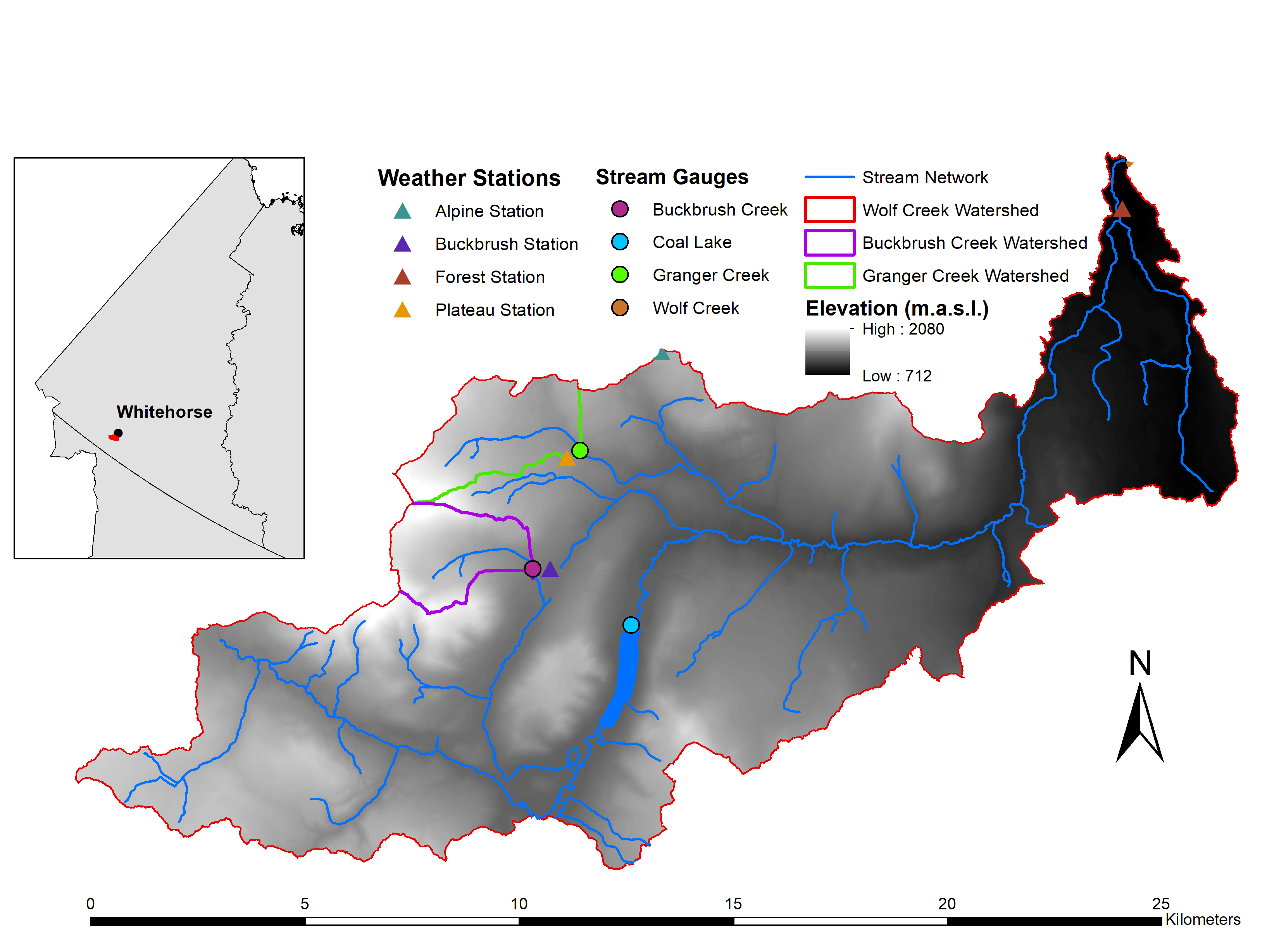
As I mentioned in my previous blog post, there have been no full classifications of the WCRB since 1997 1 despite observed changes. For my updated classification, I will be combining terrain and vegetation derivatives from a high-resolution LiDAR survey from August 2018 along with a 4-band WorldView-2 satellite image purchased from DigitalGlobe.

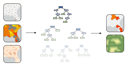
The Random Forests supervised machine learning algorithm 2 has become a widely used classification approach for fusion of several high-dimensional datasets in remote sensing and other fields. 3 This is an ideal approach for my project, as LiDAR and multispectral imagery both contain valuable information on vegetation and landscape properties.
Though the Forest-Based Classification and Regression tool exists in ArcGIS Pro, we’ve decided to use the randomforest package in R Statistics 4 to maintain consistency with the current literature. This provides me an opportunity to further explore the R-ArcGIS bridge as it now supports raster data (as of May 2018).
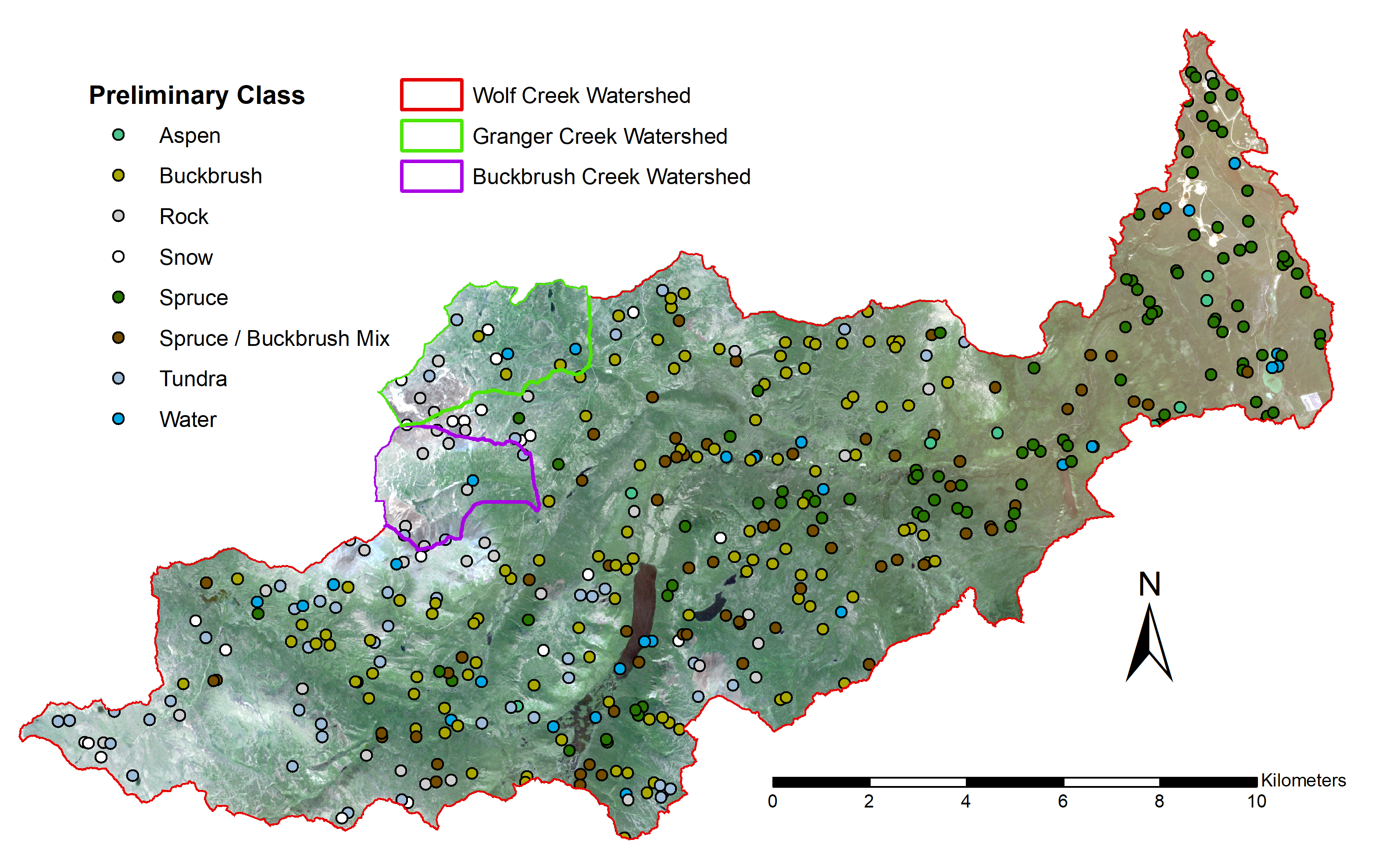
I’ve been working through preliminary classifications to help figure out how many classes we can accurately tease out of the data before I head to the field in a couple weeks, working along with a great tutorial from Wageningen University and Research. After preparing all my individual rasters and training/validation points using a combination of ArcGIS, LAStools, and SAGA GIS, these can be imported into R using the R-ArcGIS bridge and stacked to create a RasterBrick object (analogous to a multi-band raster in ArcGIS) to explore. For example, the graphic below shows the relationships between different Sentinel-2 bands and a LiDAR DEM of the study area, created with one line of code using the pairs() function in the raster package.
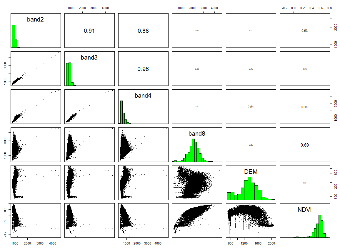
All of this pre-processing can either be done in ArcGIS or R before performing the classification, so having the option to seamlessly transfer back and forth using the R-ArcGIS bridge can be very time-saving especially if you’re not as experienced with R scripting yet.
Another important part of classification work is the collection of training and validation data in the field. A large, well-distributed ground truthing network is essential to performing a quality classification of any kind 3. This summer, I’ll be using the Collector for ArcGIS app to help navigate around our ~180km2 study area and log ground truthing points. As one of my colleagues at Mac described in an earlier blog post, this app allows you to collect spatial data in the field without needing WiFi or cellular data, and automatically uploads it to ArcGIS Online once connected again.
After identifying potential ground truthing sites throughout our study area using the Create Random Points tool, I can upload these along with a map of the WCRB to ArcGIS Online for navigation purposes. In the field, I’ll be recording potential land cover classes and taking photos of each site using the app. Once we get back to WiFi, I’ll type up my field notes of site descriptions and append them to each point and photo that’s already uploaded to ArcGIS Online.
I’m excited to get back in the field this June, collect some cool data, and use it to produce something useful for future WCRB studies in the lab. There’s a ton of other things to do in the field that I haven’t mentioned yet including validation of our two LiDAR datasets, georectification, and quantifying vegetation change. Stay tuned for more posts!
Work Cited
1) Francis, S. (1997). Data Integration and Ecological Stratification of Wolf Creek Watershed, South-Central Yukon. Applied Ecosystem Management Ltd.
2) Breiman, L. (2001). Random Forests. Machine Learning, 45, 5–32.
3) Millard, K., & Richardson, M. (2015). On the importance of training data sample selection in Random Forest image classification: A case study in peatland ecosystem mapping. Remote Sensing, 7(7), 8489–8515. https://doi.org/10.3390/rs70708489
4) Liaw, A., & Wiener, M. (2002). Classification and Regression by randomForest. R News, 2(December), 18–22. https://doi.org/10.1177/154405910408300516