
Spatial statistical analysis of African conflicts
Spatial statistical analysis of African conflicts
What trends can we uncover given the traits of actors, such as nations, and information on a phenomenon of interest, such as violent conflict? What methods can be used to establish relationships between a study phenomenon and variables that can potentially be used to explain such trends? Are the results these techniques yield valid, or simply the product of random chance or systematic design? And if all proceed, what purpose do the findings serve? Do relationships conform to or contradict prevailing theories? Herein discussed are the findings of a course project completed for Geography 4GA3 at McMaster University with Dr. Antonio Paez and Patrick Deluca that sought to answer these questions.

The data used for this analysis were sourced from the conflict and Peace Data Bank (COPDAB) published in 1980, compiled by Edward E. Azar and associated students at Stanford University, Michigan State University, and University of North Carolina at Chapel hill. The data bank is a longitudinal collection of over half a million events with recorded variables for the “actions, reactions, and interactions between nation states.” Such events represent a comprehensive record of incidences that include wars, agreements, mobilizations, diplomatic visits, blockades, etc., and are highly useful for analysis.
Spatial statistical analysis often begins by first visualizing (e.g., Figure 1) and exploring the data under evaluation. An Esri product that greatly aids in the exploration process is the exploratory regression tool found in ArcGIS Pro. This tool performs regression analyses iteratively for all possible combinations of explanatory variables, within the parameters specified by the user (R-squared, p value, variance inflation factor, Jarque Bera p value, spatial autocorrelation p value). A partial sample of the output from this tool is shown in Figure 2, listing the models with the highest R-squared values of all the possible combinations for 4 explanatory variables, and under the heading ‘passing models’ those which met all the criteria indicated by the user are listed.
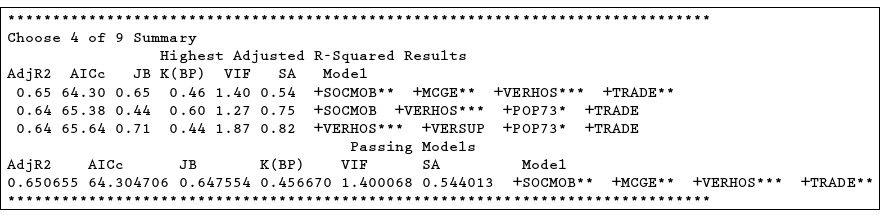
What is known about the data at this point in the analysis? A lot, actually… but there is work yet to be done, and depending on how other statistical tests return, possibly much more. At each number of variable combinations in the exploratory regression an R-squared value, or coefficient of determination, is being reported between 0.50 and 0.70. That is, between 50% and 70% of the variation in the total conflict index can be predicted by certain combinations of explanatory variables. This result indicates our data are useful and are not simply a collection of unrelated factoids. However, is the degree to which variables can predict the total conflict large enough to be considered ‘significant’, or small enough to be considered noise or the product of random chance? As exploratory regression also returns the models that passed all criteria, and one of those criteria is a user-specified p-value (in this case, the standard 0.05 or 5% threshold), we can conclude that the data are both useful and statistically significant.
Thus far determined through the exploratory regression tool in ArcGIS Pro is that the data are of use, and that a working model of the relationship between conflict and predictor variables can be derived. One of the initial questions has been answered, that results are not the product of random chance, but what about systematic design? A spatial linear regression makes a number of assumptions about the distribution and patterns within the study data that have yet to be verified through diagnostics. These are the standard assumptions for a linear regression of linearity of the relationship between dependent and independent variables, along with the homoscedasticity, independence, and normality of the residuals. Once tests have been performed to assure these assumptions have been met, and the analysis will not require a spatial lag model to compensate for spatial autocorrelation, it can be assured that the systematic design is not responsible for the model results.

Given a working model that meets all the criteria for a valid linear spatial regression, what does the model tell us? According to the signs associated with each variable, as the verbal hostility index, total trade, military expenditures, and social mobility all increase, a greater amount of total conflict can be expected. Two of these variables, the verbal hostility index and military expenditures are self evident – it’s reasonable to assume that more military expenditures and hostility in a nation will be associated with more conflict (this does not however serve as any indication of whether one precipitates the other, or causation). The other two variables are where things get tricky, as they are contrary to the prevailing theories in the literature which in themselves are not crystal clear. There has long been a sentiment that greater trade between nations enhances cooperation and fewer conflicts should follow. Warring costs money though, as is directly represented by the military expenditures variable – and rarely does a nation produce all the goods needed to wage a conflict. Instead they must be acquired through trade. There is also the consideration that the literature speaks to the overarching global condition, and not directly to the conditions in Africa in the 1960s and 70s as we are trying to address here. The social mobility index being correlated with conflict is likewise curious. This index reflects the degree to which individuals in a nation are free to move between social classes. Generally a greater social mobility is regarded favourably, as the poor are afforded opportunity to move into the middle class, having a positive effect on the national economy (perhaps where greater trade comes into play) and is considered a stabilizing force for democracy as more of the citizenry has a stake in the success of the nation. However democracy is not the prevailing system among these actors, and there is also the consideration that downward movement in social classes could also be responsible for greater social mobility and the discovered trend. This is where the use of historical data can become challenging, as a review of the available associated literature does not indicate what exactly these variables represent or how they are coded. One can only review the other literature and try and make a best guess as to what is responsible for the trend that we see.
The findings of this analysis are interesting and spur a myriad of questions well beyond the scope of this work. What we know for certain is that the variables chosen for a final working model of total conflict in the 44 African nations surveyed from 1966 to 1978 can in fact predict most of the variation in conflict, are statistically significant as to not be attributed to random chance alone, and comply with the assumptions of linear regression. Performing such analyses provides us insight into the relationships between different phenomena in a system that are otherwise difficult to establish, and Esri products such as the exploratory regression tool can greatly aid the analyst in the process. My hope in writing this blog post is to offer a small highlight in the power of spatial statistics. If you are a GIS or geography student planning your upper years of coursework, I would highly recommend taking a class on the topic.