
Using Optical Imagery and Fuzzy Logic to Map Wildfires in British Columbia
Exacerbated by human-induced climate change, wildfires have become increasingly severe and devastating in recent years. In British Columbia over the past decade, wildfires have consistently cost hundreds of millions in damages and pose serious health threats to the population as the smoke lingers over populous areas throughout the province.
For our British Columbia Institute of Technology (BCIT) Project sponsored by Planetary Remote Sensing, myself, Brent Strong and Brad Markinkow aim to detect and map recent wildfires in British Columbia (B.C.) using a combination of remote sensing data from radar and optical satellites. The project will explore various image classification techniques and work towards building a series of Python scripts to automate the delineation of burned areas after wildfires.
This blog post will give an overview of how we’ve utilized publicly available optical imagery from the European Sentinel satellites to build a framework to map out burned areas with fuzzy logic.
Gathering Data
Various 2021 wildfires in B.C. were chosen as areas of interest for our project. The Tremont Creek fire west of Kamloops burned over 62,000 hectares from July until September. We used The Copernicus Open Access Hub to download pre-fire and post-fire raster images of the Tremont Creek fire (Figure 1).
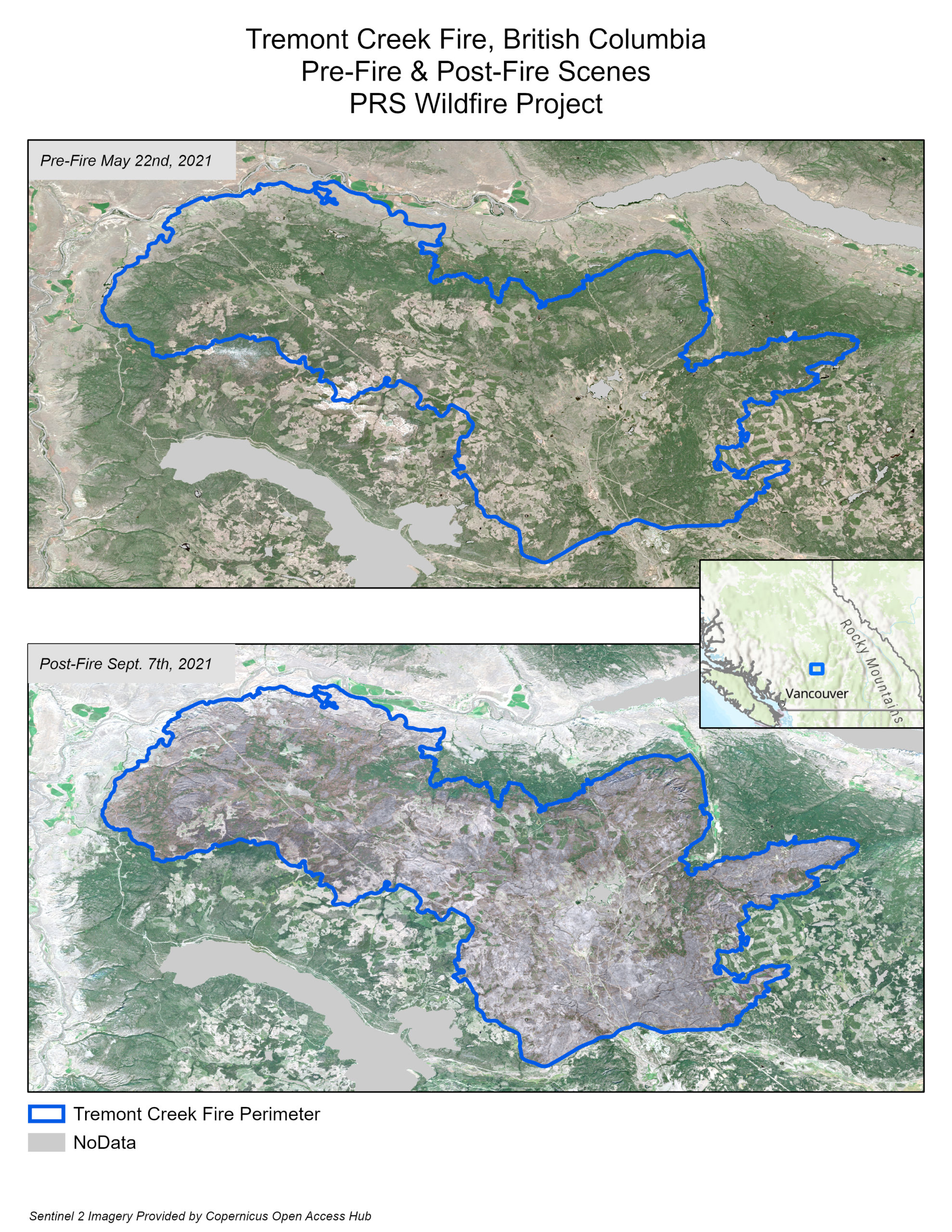
Figure 1: Tremont Creek pre-fire and post-fire scenes
Raster Dataset Creation
Optical imagery is supplied from The Copernicus Open Access Hub as separate JPEG 2000 (.JP2) files for each band of optical data. These files exist at varying resolutions (Figure 2). In order to work with this dataset in ArcGIS Pro, these separate raster band files have to be merged into one raster dataset. To handle this task, a simple Python script was created to resample all of the bands down to 10 meter resolution using the Resample ArcPy tool before merging all bands into a single raster dataset using the Composite Bands tool in ArcPy.
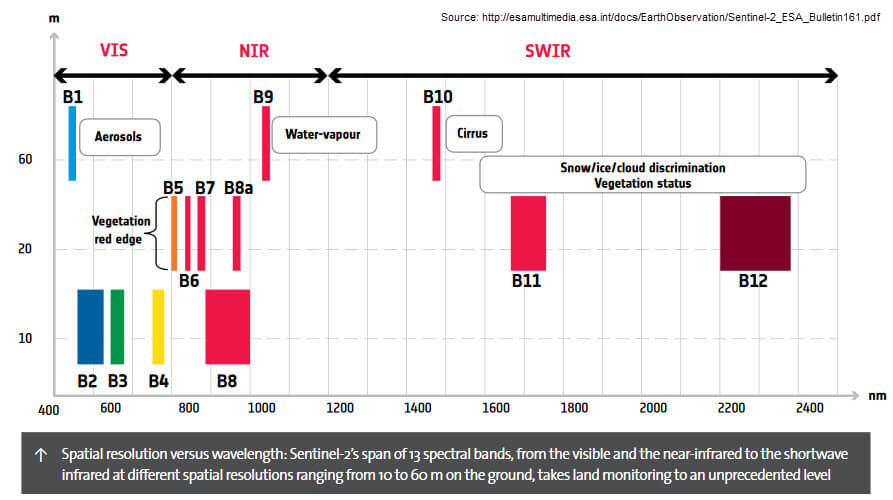
Figure 2: Sentinel Bands, with band wavelength in nanometers on the X-axis and image resolution in meters on the Y-axis (Sourced from: https://brooks.eco/projects/mapping-wetland-vegetation-from-sentinel-2-satellite-imagery_117s38)
Generating Spectral Indices
The next step involves using our raster datasets to generate layers of spectral indices that illuminate burned areas. Spectral indices are combinations of the pixel values from two or more spectral bands in a multispectral image. Spectral indices are designed to highlight specific phenomena that are taking place on the surface. Variations in the surface reflectance at different wavelengths across the electromagnetic spectrum can be exploited to highlight these changes (Figure 3). The Normalized Burn Ratio (NBR, Figure 4) is one index that is specifically tailored for mapping burned areas and quantifying burn severity. Other spectral indices that are meant to monitor vegetation productivity, such as the Normalized Difference Vegetation Index (NDVI), are also useful for for these purposes.
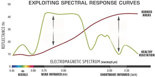
Figure 3: Spectral signatures for burned areas and healthy vegetation (source: https://un-spider.org/advisory-support/recommended-practices/recommended-practice-burn-severity/in-detail/normalized-burn-ratio)

Figure 4: Normalized Burn Ratio equation (source: https://un-spider.org/advisory-support/recommended-practices/recommended-practice-burn-severity/in-detail/normalized-burn-ratio)
Spectral indices can be easily created in ArcGIS Pro by combining separate raster bands together using the Band Arithmetic tool or with Raster Functions. A second Python script was created to take the output from the first script and generate new raster datasets of spectral indices. By subtracting pre-fire spectral index rasters from the accompanying post-fire spectral index rasters, we can highlight landscape changes caused by wildfires. In addition to NDVI and NBR, other spectral indices such as the Char Soil Index (CSI), the Mid Infrared Burn Index (MIRBI) and the Relative Burn Ratio (RBR) were generated. Results for NDVI (Figures 5 and 6) and NBR (Figures 7 and 8) are shown below.
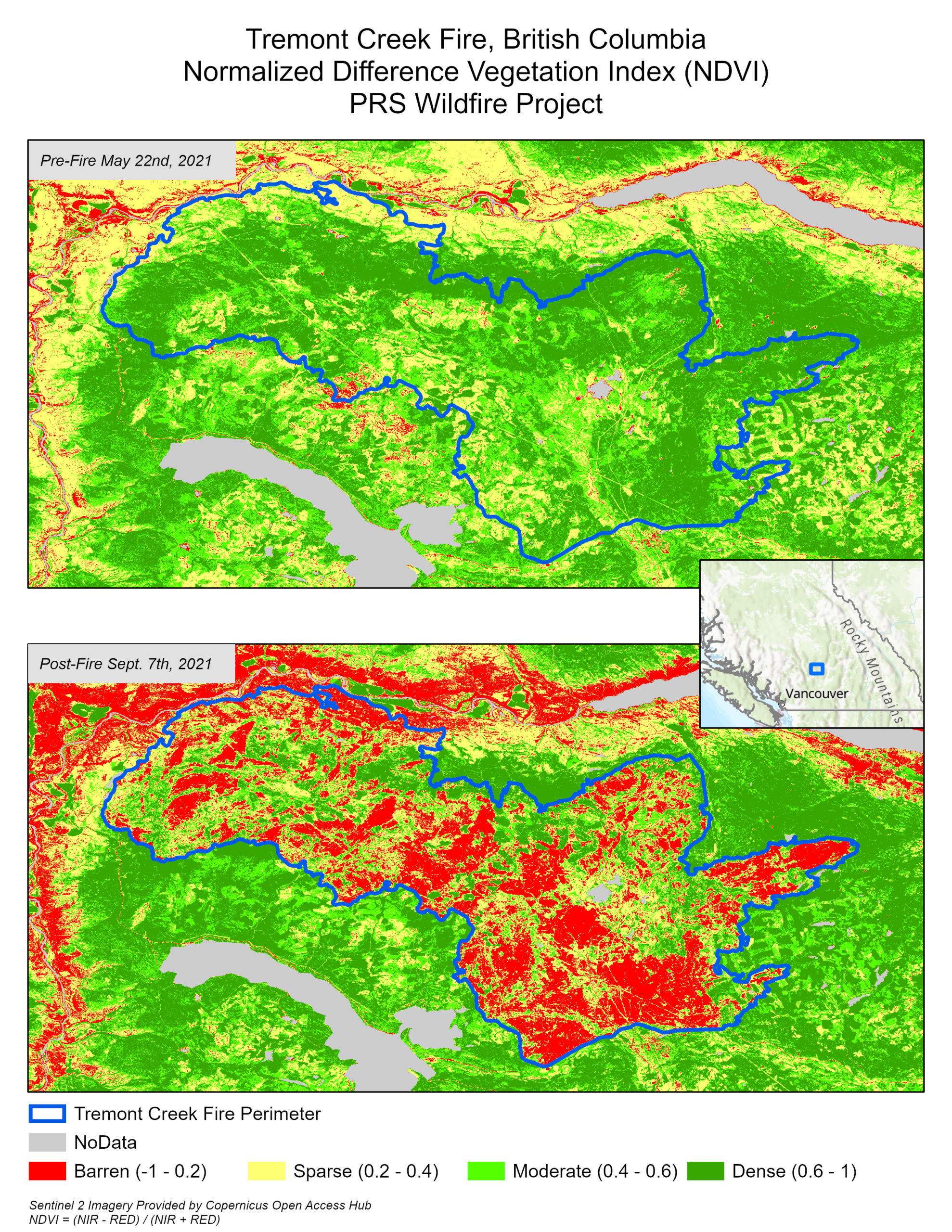
Figure 5: Tremont Creek change in Normalized Difference Vegetation Index (NDVI)
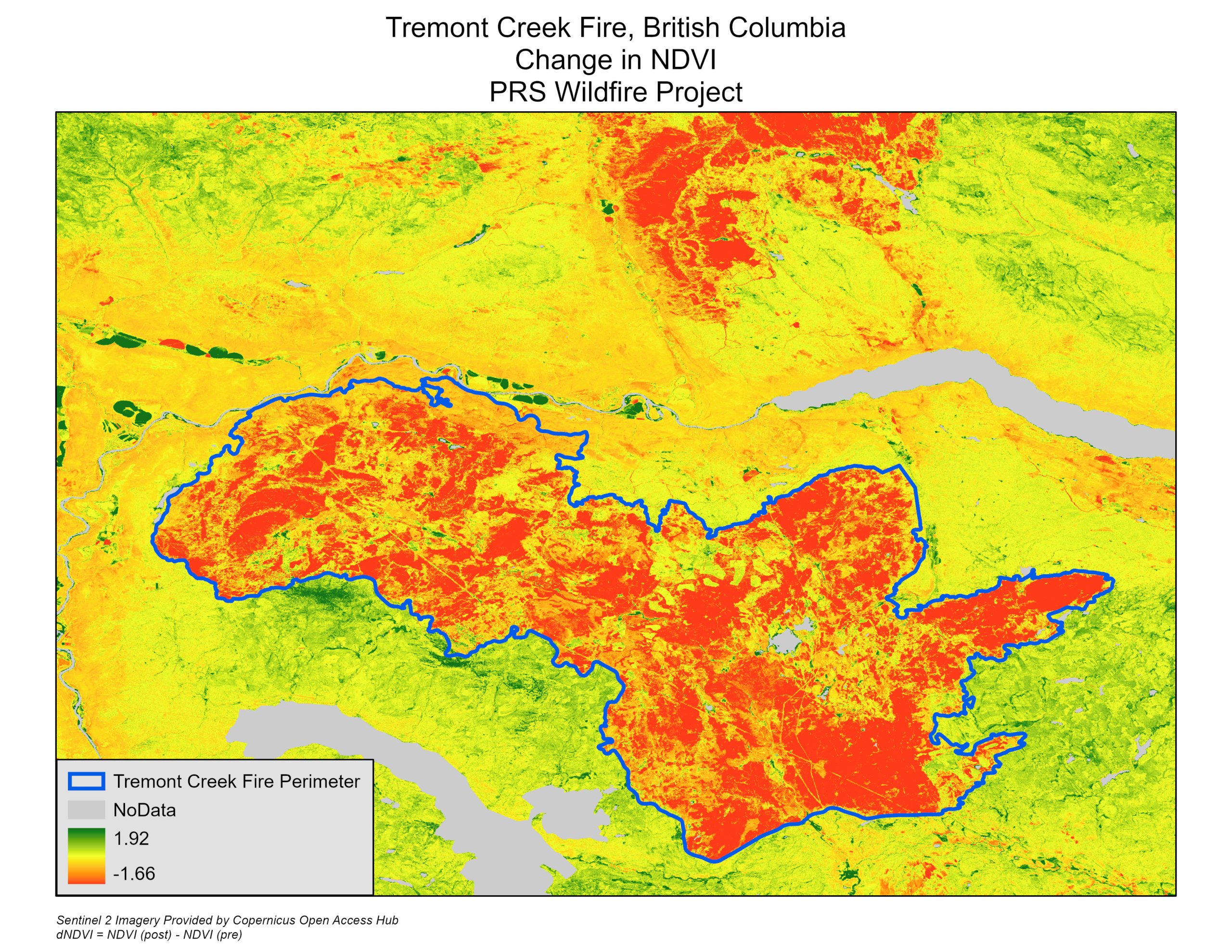
Figure 6: Tremont Creek change in NDVI (Post – Pre)
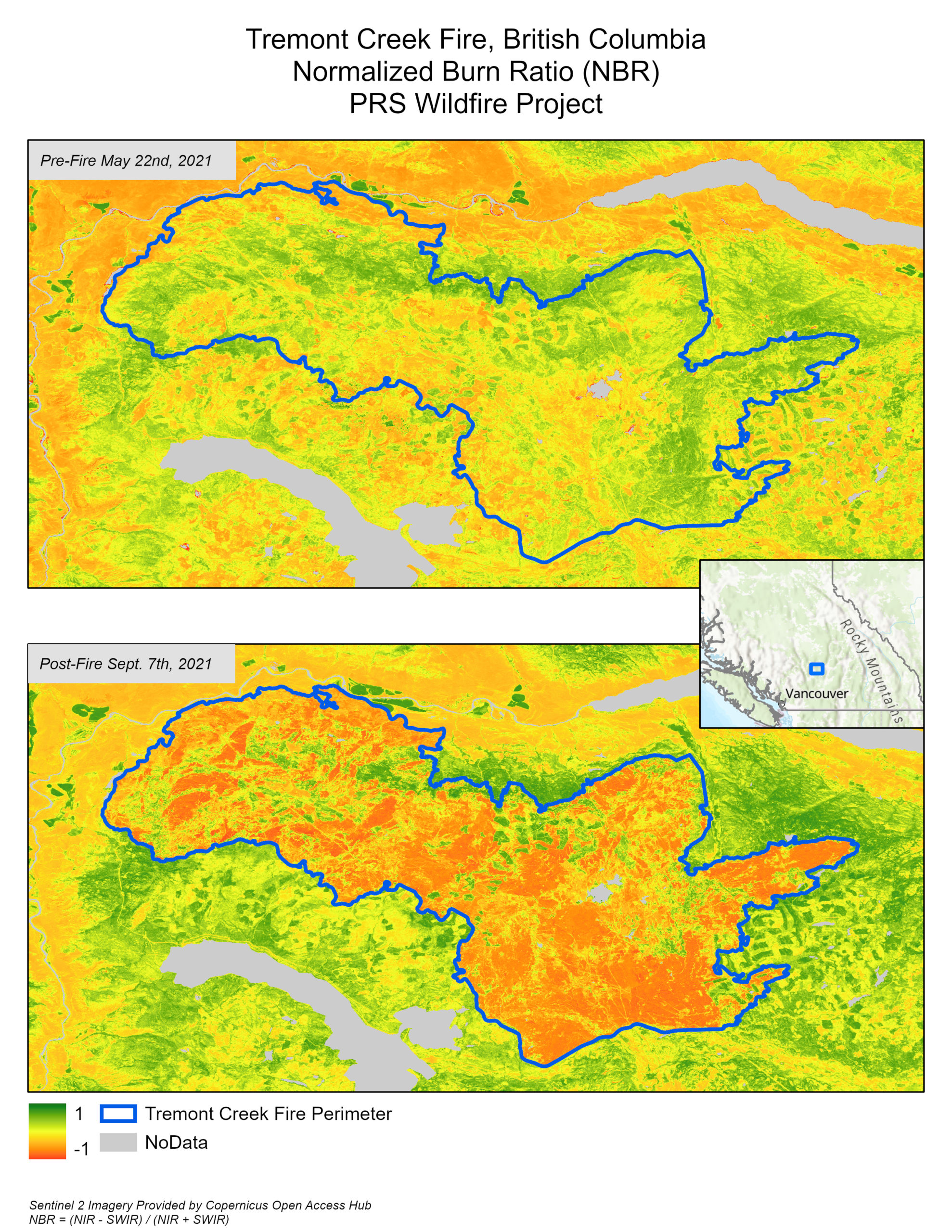
Figure 7: Tremont Creek pre-fire and post-fire Normalized Burn Ratio (NBR)
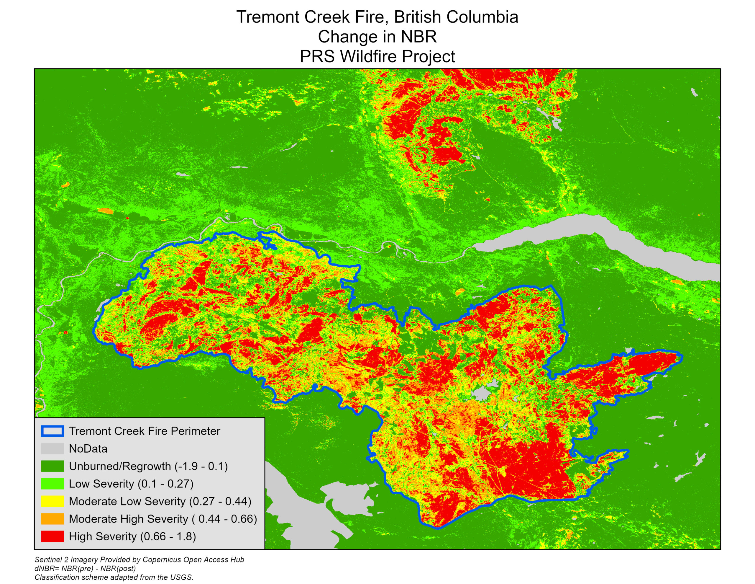
Figure 8: Tremont Creek change in Normalized Burn Ratio (dNBR)
Fuzzy Logic
The next step in our analysis will be to determine burned and unburned pixels in our scene using Fuzzy Logic. Traditional image classification and overlay techniques are based on pixel values being within a class or outside that class. Fuzzy Logic defines how likely it is that the pixel is a member of a class and addresses situations when the boundaries between classes are unclear (source). The process of applying fuzzy logic entails overlaying our spectral indices rasters onto one another in order to determine the possibility that each pixel is contained in the class of burned pixels.
The evidence of a burned area provided by each spectral index layer is quantified by using fuzzy membership functions. We used the Fuzzy Membership tool to apply a linear function to the input spectral index values to transform the inputs into new ‘fuzzified’ rasters with normalized values on a 0 to 1 scale. Pixel values of 1 indicate full certainty that the pixel value is in the burned class, and a value of 0 indicates with full certainty that the pixel is not in the burned class.
These fuzzified rasters are then used as inputs to the Fuzzy Overlay tool in ArcGIS Pro. The Fuzzy Overlay tool determines the likelihood of a cell being a member of a class by using all of our fuzzified spectral indices as selection criteria. After applying a threshold value of 0.7 to the results we can see that the Fuzzy Overlay layer does a reasonably good job at delimiting newly burned areas (Figure 9).
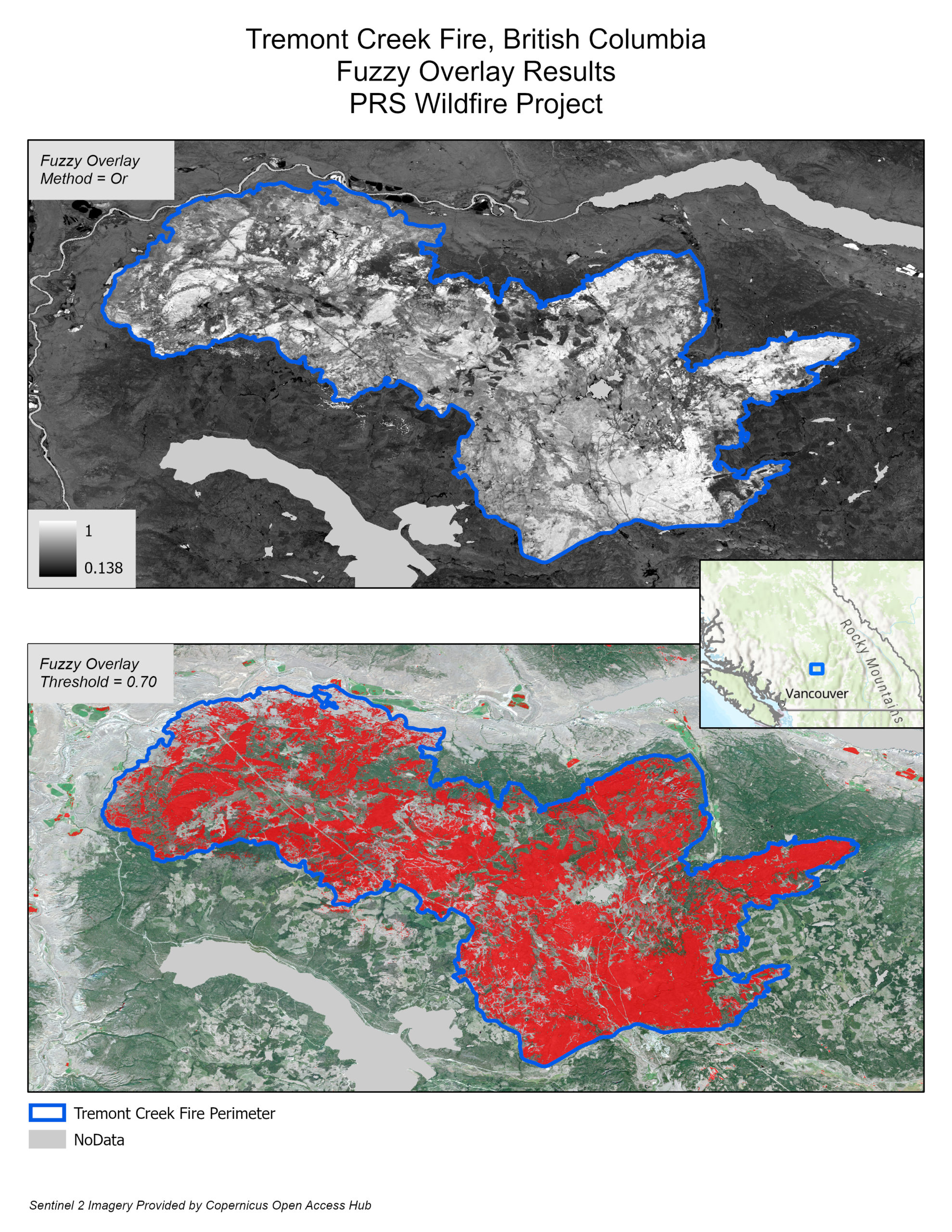
Figure 9: Fuzzy Overlay results
Conclusion
While the results are promising for our project, they also illuminate limitations of this workflow. One such limitation is that the existence of false positives and the overall accuracy depends on the chosen threshold value. Additionally, the minimum value from the Fuzzy Overlay results is approximately 0.138, which indicates that no pixel in the image was determined to be unburned. We know that to be false. The analysis workflow is also dependent on clear satellite images free of cloud cover. In future work, we will refine our fuzzy logic methodology and incorporate data from Synthetic Aperture Radar images into our image classification analysis.