
Analyzing the Best Tourism Spots
This blog post is about part of my GIS assignment from last term. The objective of this part was to teach us how to use viewshed analysis and least cost path analysis to find the best tourism spot (out of three candidate spots) based on how much of the city/urban-areas are visible from that particular spot and how easy/difficult the tourism spots are to reach from the urban area. The criteria for difficulty to reach was based on the slope of the area as well as the land cover type (developed, grassland, forest, shrub, etc.) with water being impassable, the easiest hiking route being the one that is the flattest with the most easy-to-traverse land cover types in a 50/50 weight ratio.
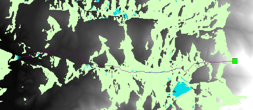
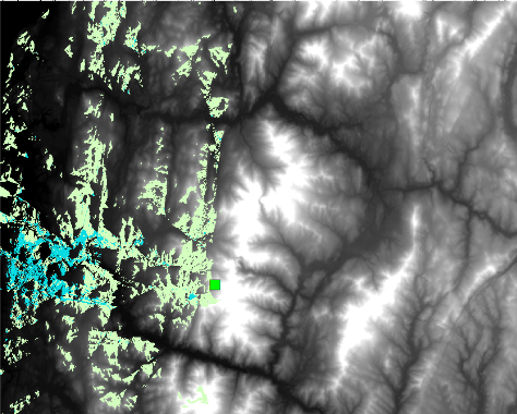
To accomplish these two tasks, we were given three candidate sight-seeing spots, the DEM file, and the landcover types. I initially performed a viewshed analysis to identify all areas that were visible from each of the candidate spots based on the DEM file which contains altitudes of all points in the area. I then used the landcover types to create new dataset that includes only areas that are both viewable and classified as urban landcover for each candidate spot. Since all three of the viewable urban datasets had the same units, I was able to determine which candidate spot was the best by calculating the largest area of viewable urban areas, according to the number of units for each. After I found the best candidate spot, I created a least cost path to the location using the cost path as polyline tool, using both DEM and landcover type datasets.
Another part of this assignment required us to create our own custom geoprocessing script tool for ArcGIS using a Python script. We were tasked to create a tool that would turn a feature class into points, then create buffers around the points. The tool needed to be configured to accept input parameters (e.g., the points), and provide an output parameter for the resulting buffers.
This assignment is probably the most challenging one I’ve come across so far, the instructions given were quite vague and steps to proceed were not the most clear. A large portion of the data that we were given had to be reclassified and prepped too, before they were usable for analysis purposes. While I can’t share the detailed steps for this assignment, i think it was a great experience that exposed me to problems that are quite realistic (e.g., finding the easiest path to a location), and taught me sill that will be useful in my future.