Evaluation of influential variables on Calgary’s dwelling price (Spatial Autoregressive Model)

Faculty of Art, Department of Geography, University of Calgary

Geography 639: Final Project, Winter 2024

Abstract

The prediction of dwelling values can identify the imbalances between the dwelling supply and residents’ demands as well as the communities’ needs. This project aims to describe the relationship of some influential socio-economic variables on the median value of dwellings in Calgary based on the community census data (2016). Multivariate linear and spatial regression models are applied to evaluate the association between this dependent variable and five independent variables namely population density, mean traffic volume, ratio of post-secondary, median household income and area of commercial uses. The final outcomes reveal that two variables “population density” and “log area of commercial uses” affect dwelling prices negatively. However, the ratio of educated people is positively associated with dwelling values. The comparison of the two models represents that the SAR model with a pseudo-R-square of 0.32 has better performance while it reduces the spatial autocorrelation in residuals compared to the linear model having a R-square value of 0.29.

Introduction

Many households have a large chunk of their wealth invested in their homes. Housing is considered a highly heterogeneous good varying across different dimensions (Lectures on Housing Economics: A European Text, n.d.). Housing value can be impacted by a combination of factors: structural features, economy, demography, location, etc. For instance, “the expansion of roads results in more traffic noise having a detrimental effect on the value of adjoining residential properties” (The Impact of Transportation on Real Estate Values, n.d.). Accordingly, multivariate spatial regression analysis is applied to answer the following questions: Is Calgary’s dwelling price significantly associated with some socio-economic factors? To what degree, do the variables affect the housing price? Does the dwelling value show positive spatial autocorrelation over space? Does the Spatial Autoregressive Model (SAR) reduce the spatial autocorrelation of residuals? I expect that the population density and area of the commercial uses show high positive coefficients. Conversely, the traffic volume and the ratio of postsecondary will have a negative and a trivial correlation with Calgary’s housing values respectively. Moreover, I assume that dwelling values represent positive spatial autocorrelation in Calgary, indicating similar attributes (dwelling price) tend to be clustered in the city. Using a standard linear model will culminate in spatially autocorrelated residuals making the prediction of dwelling values unreliable, as a result by using the SAR model, I hope the spatial autocorrelation in residuals will be decreased. In addition to that, the pseudo-R-square acquired from the SAR model is higher compared to the linear model showing the model can capture more variability of data.

Methods

The data is based on a community profile in 2016, and there are 202 observations. Three observations have no report for median HH income, so zero is entered for their values. Moreover, the “area of commercial uses” has 33 records of zero. After checking the location of the communities, I understood that these communities either are residential zones or are at the peripheral edge. Calgary’s median dwelling value is a dependent variable (DV). There are five independent variables (IVs): population density, mean traffic volume, the ratio of post-secondary, median household income and area of commercial uses. To ascertain the relationship between a group of IVs and a single DV, multivariate linear and spatial regression models are performed. “Spatial regression specifications are most useful to researchers seeking to either investigate a spatialized version of a dependent or independent variable or account for spatial autocorrelation observed in data that would violate traditional regression assumptions”(Sauer & Stewart, 2023). By applying the Spatial Autoregressive Model (SAR), I can evaluate how a combination of five variables impacts the dwelling values quantitatively while simultaneously addressing spatial autocorrelation. There are three general steps to achieve the objectives. The first step is preprocessing to evaluate the data and variables in terms of their distribution, gaps, and spatial autocorrelation of DV using Moran’s Index. Afterwards, I run the standard regression model using the Ordinary Least Square (OLS) estimation. The next step is to evaluate the acquired residuals in terms of their distribution (Shapiro-Wilk’s W test), spatial autocorrelation (the Lagrange Multiplier Test), and heteroscedasticity (the Studentized Breusch-Pagan Test). The results of the Lagrange Multiplier Test aid me in identifying whether I should apply SARlag or SARerr based on the presence of spatial autocorrelation and the significance of that. After running the proper SAR model with backward selection, the residuals should be tested again whether the spatial autocorrelation has decreased. Finally, by calculating the Pseudo R-square I can compare my SAR model with the Standard Regression Model, provided that the number of variables is the same.

Results

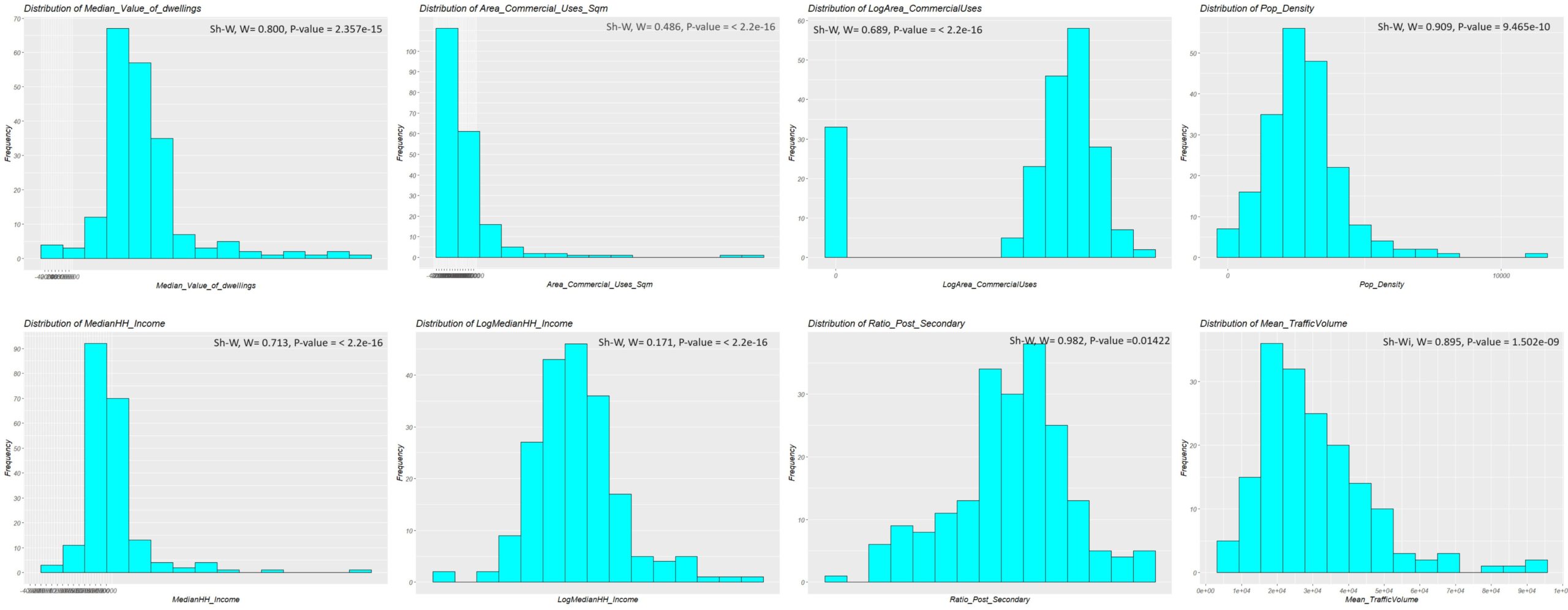
Based on Figure 1, the distributions of “median value of dwellings” (DV), “mean traffic volume”, “ratio of post-secondary” and “population density” are approximately normal. On the other hand, two variables called “area of commercial uses” and “median income of households” have Poisson and right-skewed distributions respectively. I applied logarithms to these variables to make them close to normal (quasi-normal) distribution. According to the Shapiro–Wilk test results, all the p-values of the variables are below the significant level indicating the rejection of the null hypothesis meaning the data do not follow a normal distribution. Sometimes there might be a difference between a visual evaluation and a quantitative assessment (Shapiro–Wilk test) because quantitative assessments can capture outliers and slight skewness.

There is no high correlation among variables (Table 1 and Figure 2), meaning I can enter all the variables into both initial models and perform backward selection.

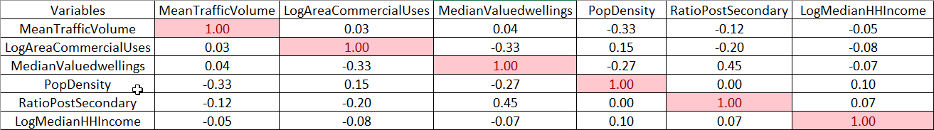
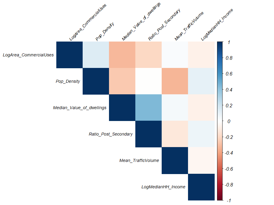
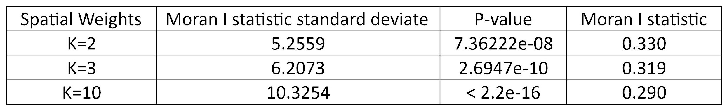
Table 2 represents the results of spatial autocorrelation of DV (dwelling prices) using different spatial weights. The two nearest neighbours seem to capture more spatial autocorrelation with a value of 0.330, also considering the P-value of 7.36222e-08, the dwelling values are positively spatially autocorrelated. Additionally, the Z test (5.255) is higher than the critical value of 1.96 verifying significant spatial autocorrelation.

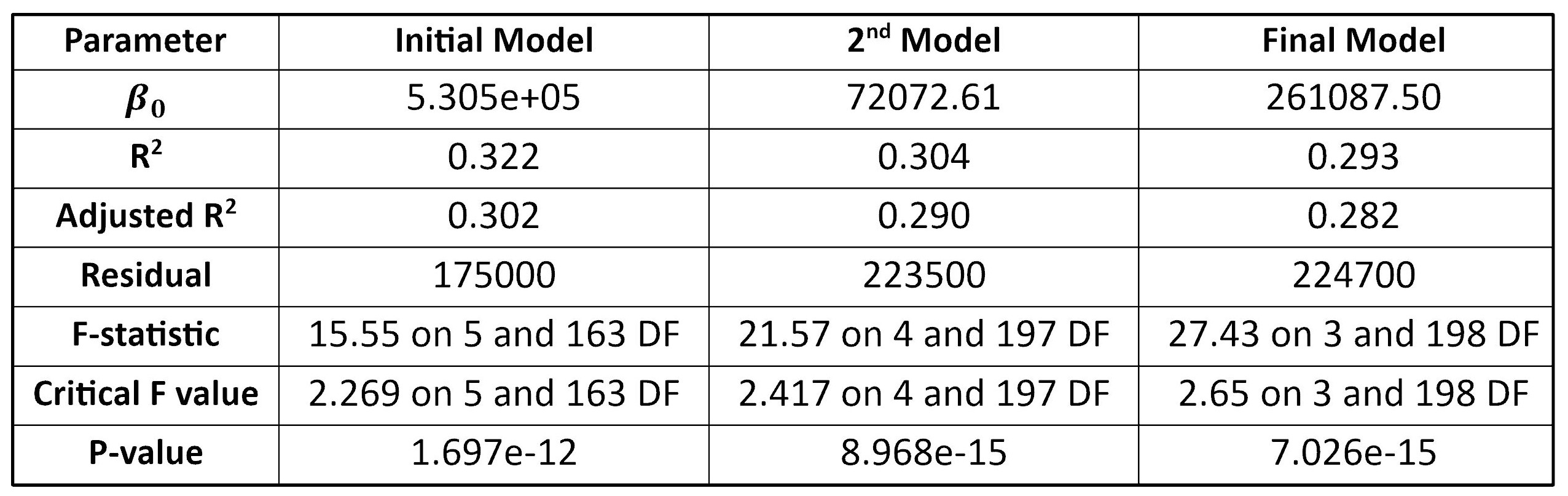
In the initial standard linear regression model with five independent variables, “Mean_TrafficVolume” has the lowest t value, so it is removed as a non-significant variable. In the second mode, “LogMedianHH_Income” is a non-significant one. Accordingly, the final standard regression model has three significant variables having Pr(>|t|) lower than the significant level namely “Pop_Density”, “LogArea_CommercialUses” and “Ratio_Post_Secondary” with the coefficients of -43.06, -12557.21 and 974263.25 respectively. Considering adjusted R-square values, the initial model with a value of 0.302 represents a better goodness-of-fit however the final model has the highest F-statistics (Table 4).

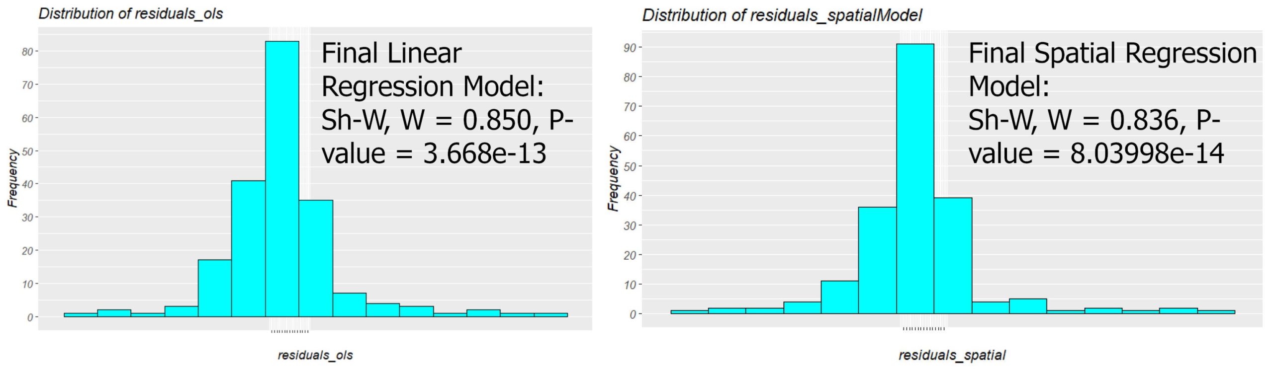
The residual histogram of OLS estimation shows a normal distribution; however, the P-value (3.6677e-13) of the Shapiro-Wilk normality test is lower than 0.05 representing the departures and deviations from normality (Figure 3).

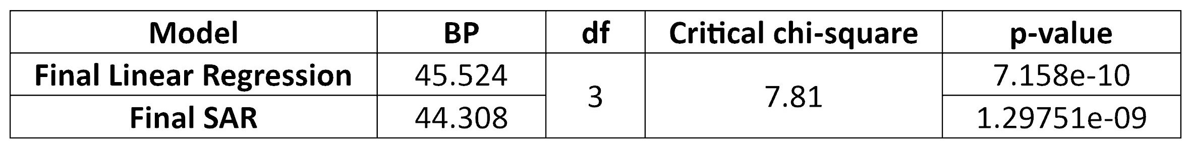
According to Table 3, residuals of the final linear model indicate heteroscedasticity because not only is the BP test value (45.52) higher than the critical value of chi-square (7.81) for a degree of freedom three but also the P-value is < 0.05 resulting in rejection of the null hypothesis of homoscedasticity, so there is significant heteroscedasticity.

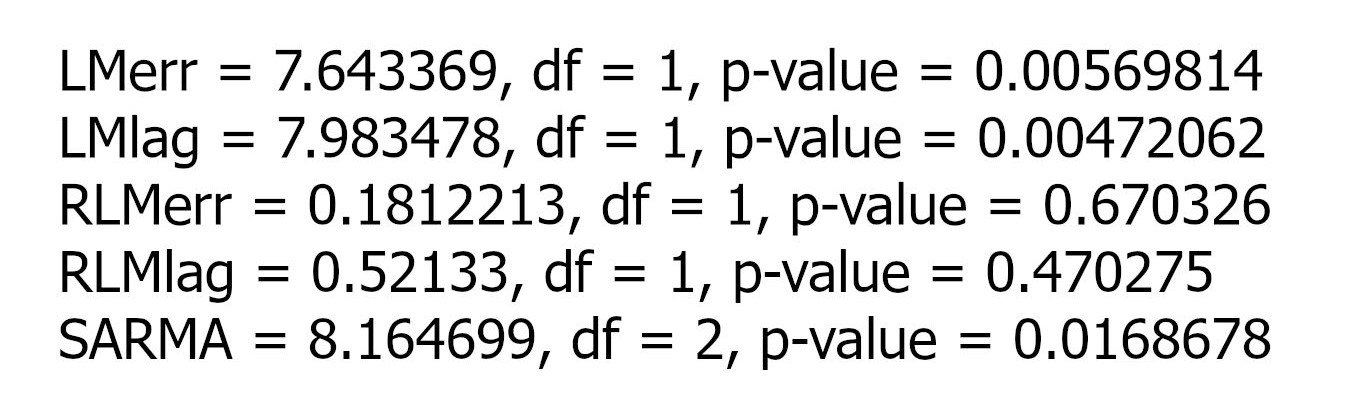
The Lagrange Multiplier Test (Figure 4) reveals that both LMerr (value of 7.64) and LMlag (value of 7.98) models are significant considering the critical value of chi-square with one degree of freedom and P-values. Therefore, there is spatial dependence both in the DV and residuals of the model, however, I choose the spatial lag model (LMlag) because it appears more significant with a value of 7.98. The initial spatial lag model is performed with five independent variables, the results show that the absolute Z values of “Mean_TrafficVolume” and “LogMedianHH_Income” are 0.18 and 1.53 indicating the least significant variables.

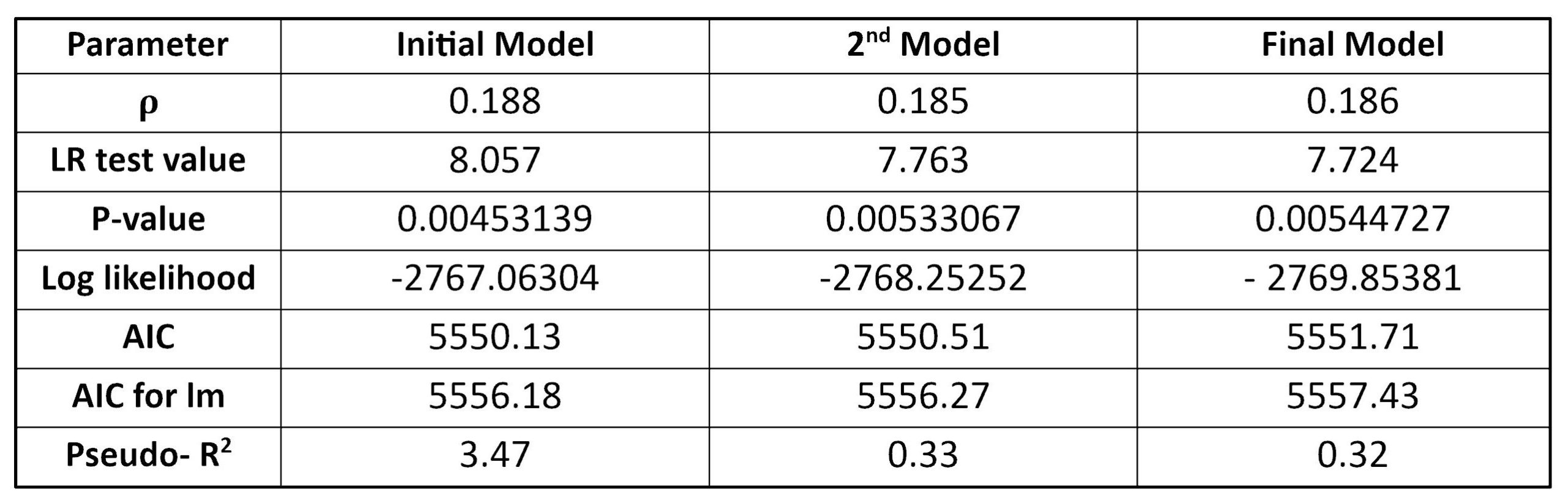
Based on Table 5, the Rho value of -0.129 indicating the correlation coefficient between the dwelling price and its spatial units is not significant. The initial SAR model is not statistically significant because the likelihood ratio (3.83) < critical chi-square (11.57) and the P-value (0.050236), so I fail to reject the null hypothesis. “Mean_TrafficVolume” and “LogMedianHH_Income” will be omitted for the second and final model successively due to non-significancy. The correlation coefficient in the final model has a value of 0.186 showing no significant spatial dependency between DV and neighbouring areas. The final spatial model has a likelihood ratio of 7.724 < the critical chi-square value with three degrees of freedom (7.81), but the P-value (0.00544727) is lower than the significant level so I reject the null hypothesis indicating the entire regression is statistically significant. Three variables “Pop_Density”, “LogArea_CommercialUses” and “Ratio_Post_Secondary” have Pr(>|Z|) lower than 0.05 meaning all of which are significant. Pseudo-R square shows that the final SAR model can explain only about 32 per cent of the variation in a data set. As shown in Table 5, the pseudo-R-square cannot be an indicator for comparing which spatial model has better goodness-of-fit because the number of variables is different, AIC or loglikelihood can be used instead.  The initial spatial model has the lowest AIC value (5550.13) and absolute loglikelihood (2767.06) showing a better model, but the final model is refined by removing non-significant variables and is a simple model so considering narrow differences of the AICs, loglikelihood values and models’ complexity, the final spatial model would have a better performance.

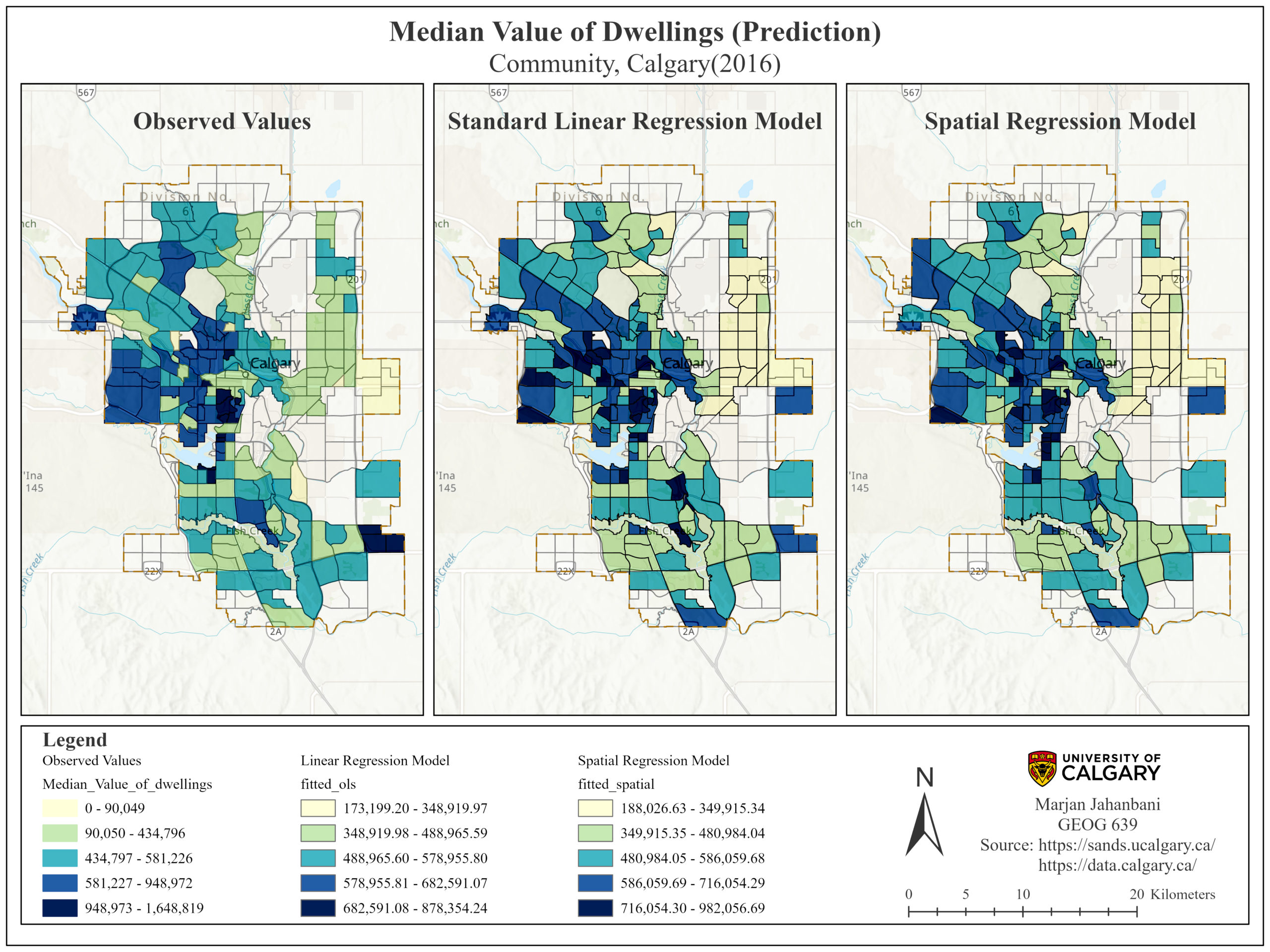
The SAR residuals seem to be normally distributed; however, the Shapiro-Wilk’s W test illustrates the data do not follow a normal distribution (P-value)(Figure 3). Table 3 reports that there is still statistically significant heteroscedasticity in the SAR residuals (P-value) which is not surprising because the spatial lag model is designed to deal with spatial autocorrelation and does not consider the non-stationarity. Finally, the Lagrange Multiplier test on the SAR residuals reports a value of 0.058 < critical chi-square (3.841) and P-value of 0.80 implying there is no spatial dependency in residuals. According to prediction maps (Figure 5), both models predict that the median value of dwellings will be high in Calgary’s western section. There are some minor differences between the two predictions. For instance, two communities located in the south are in dark blue based on linear regression (showing high median dwelling prices in the future) whereas they become pale blue in the SAR model and vice versa.

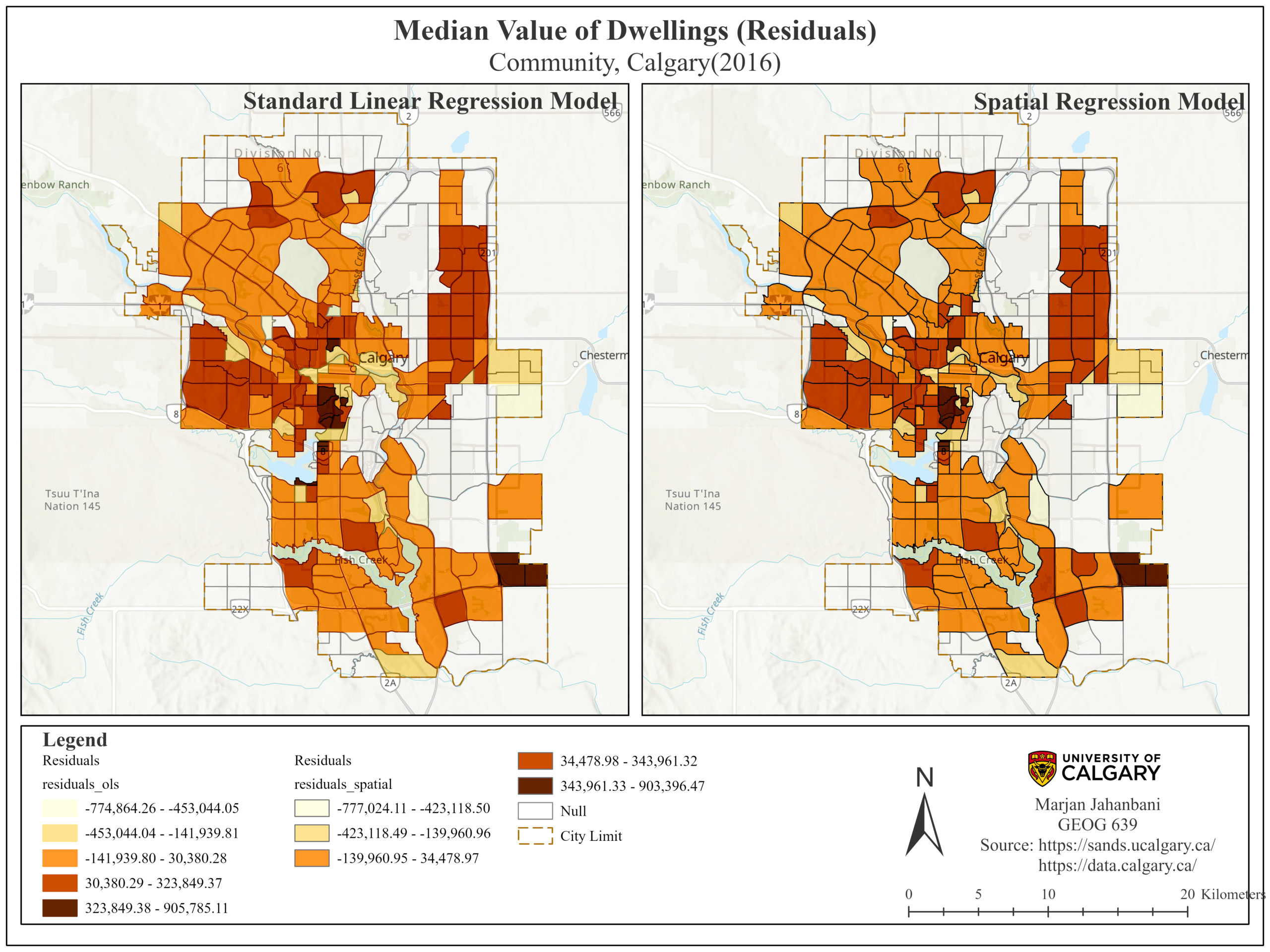
In terms of residuals (Figure 6), the SAR residuals have a range from -777,024 to 903,396 which is lower than the range of the linear model, implying the least model’s uncertainty. Indeed, linear regression illustrates poor prediction for some communities in the northwest and southwest (dark brown areas), however, the SAR residuals present those communities in reddish brown showing the level of the model’s uncertainty decreases a little bit, as a result, the SAR model’s prediction contains less amount of uncertainty compared to OLS method.

Discusssion

In response to research questions: Is Calgary’s dwelling price significantly associated with some socio-economic factors? The two final models both have three variables indicating “Pop_Density”, “LogArea_CommercialUses” and “Ratio_Post_Secondary” are significantly associated with the values of housing in Calgary. To what degree, do the variables affect the housing price? Population density has a negative association with dwelling prices with a degree of about 43 in both final models. Similarly, the log area of commercial uses has also a negative impact on housing prices meaning if the area of commercial uses increases by one unit, the housing values will decrease by about 12,557.21 units (OLS) or 11,431.12 units (Maximum Likelihood). However, the ratio of post-secondary has a positive association not only in linear regression (with a degree of 974,263) but also in the spatial model (with a value of 810,526).  Does the dwelling value show positive spatial autocorrelation over space? Yes, based on Moran’s I index (Table 2), not only is there positive spatial autocorrelation in dwelling prices but also it is statistically significant, meaning similar housing prices tend to be clustered over the city. Moreover, the results of the Lagrange Multiplier Test on the final linear regression model, also represent the spatial dependency in dependent variables (LMlag) in addition to errors (LMerr). Does the Spatial Regression Model (SAR) reduce the spatial autocorrelation of residuals? Yes, I performed the Lagrange Multiplier Test on both models’ residuals. In the final linear regression model, the degree of spatial dependency is 7.64 which shows a positive significant spatial autocorrelation however, it goes down and reaches 0.05 in the SAR model which is not significant (P-value). 

In addition, the hypothesis of high positive coefficients of population density and area of commercial uses is confuted because the population density and area of commercial uses show a negative association on dwelling prices.  The ratio of post-secondary was expected to have a trivial impact on dwelling values; whereas, the results show that this factor has the most positive influence on housing values among all independent variables.

Conclusion

This project applied two different regression models to predict the median value of dwellings in Calgary. Considering the results of both final models, it comes to the conclusion that the final spatial model has better goodness of fit because it exhibits the pseudo-R-square value of 0.32, indicating that the spatial regression model can account for 32 % of the variability of median value of dwellings and 68% will be unexplained. The most influential factor on the median value of dwellings is the ratio of people having post-secondary education meaning if this parameter goes up by one unit in a community, the median dwelling price is expected to increase by 810,526.22 units in that community, on the contrary, the increase in population or commercial uses affect the housing values negatively. Although by using the SAR model, the goodness-of-fit of the model is improved, there is still a large portion of unexplained variability in the data because of the non-stationarity leading to the inflated variance of the SAR residuals. In conclusion, I could only minimize the variance of residuals stemming from spatial autocorrelation by applying the SAR model.  To deal with the non-stationarity, the Geographically Weighted Regression (GWR) model can be utilized to see how the variance of the error will be reduced. 

Acknowledgement

I would like to acknowledge that this project was originally conducted for a course named Advanced Spatial Analysis and Modeling under the guidance of Stefania Bertazzon. I would like to express my sincere gratitude to her for her invaluable guidance and support throughout this project.

References

Bertazzon, S. (2024). R script “Lab Assignment 5.” Unpublished.

Chapter 3 Housing market | Lectures on housing economics: A European text. (n.d.). Retrieved March 27, 2024, from https://kkholodilin.github.io/Test_HE/ch-Market.html#sec:IntroMarket

Sauer, J., & Stewart, K. (2023). Geographic information science and the United States opioid overdose crisis: A scoping review of methods, scales, and application areas. Social Science & Medicine, 317, 115525. https://doi.org/10.1016/J.SOCSCIMED.2022.115525

The Impact of Transportation on Real Estate Values – xpertRealtyMarketing. (n.d.). Retrieved March 28, 2024, from https://xpertrealtymarketing.com/real-estate/impact-transportation-real-estate-values

The Symbiotic Relationship Between Commercial and Residential Real Estate. (n.d.). Retrieved March 28, 2024, from https://www.linkedin.com/pulse/symbiotic-relationship-between-commercial-residential-morgan-simpson-evv0c/