
Computing Catchment Areas for Bus Stops using GTFS Static Data
In this tutorial, I’ll demonstrate how to compute catchment areas, or network buffers, around transit stops in Hamilton, Ontario, using the ArcPy Network Analyst module and Hamilton Street Railway (HSR) General Transit Feed Specification (GTFS) static data from Open Hamilton.
Step 1: Import Required Packages
Let’s begin by importing the necessary packages. The urllib and zipfile packages are used to download and unzip the GTFS static data, respectively. The dotenv package is used to access environment variables. As I use ArcGIS Online routing services in this tutorial, I store my ArcGIS Online login credentials in environment variables.
import arcpy as ap
import os
import urllib.request
import zipfile
from dotenv import load_dotenv
load_dotenv()
Step 2: Download and Unzip GTFS Data
Next, download the GTFS static data for HSR for the 2025 winter season from Open Hamilton, and unzip it to a folder called “GTFS” in your home directory.
url = "https://opendata.hamilton.ca/GTFS-Static/2025Winter_GTFSStatic.zip"
filename = "2025Winter_GTFSStatic.zip"

opener = urllib.request.build_opener()
opener.addheaders = [('User-Agent', 'Mozilla/5.0')]
urllib.request.install_opener(opener)

urllib.request.urlretrieve(url, filename)
f = zipfile.ZipFile(filename, 'r')
f.extractall("GTFS")
f.close()
Step 3: Create a File Geodatabase
Create a file geodatabase to store the results, and use the GTFS Stops to Features tool to convert stop information in the GTFS data into a feature class.
ap.env.overwriteOutput = True

ap.CreateFileGDB_management(os.getcwd(), "transit_catchment.gdb")
ap.env.workspace = os.getcwd() + "/transit_catchment.gdb"

ap.conversion.GTFSStopsToFeatures(os.getcwd() + "/GTFS/stops.txt",
                                  os.getcwd() + "/transit_catchment.gdb/stops")
Step 4: Log in to ArcGIS Online
Log in to your ArcGIS Online portal. You can also use a local network for network analysis, but for simplicity and convenience, I am using the ArcGIS Online road network.
ap.SignInToPortal("https://mcmaster.maps.arcgis.com/",
                  os.getenv("id"),
                  os.getenv("password"))
Step 5: Set Routing Parameters
Set the routing parameters, specifically the network buffer size in minutes and the travel mode, which is walking.
modes = ap.nax.GetTravelModes("https://mcmaster.maps.arcgis.com/")
sa = ap.nax.ServiceArea("https://mcmaster.maps.arcgis.com/")

sa.defaultImpedanceCutoffs = 15
sa.travelMode = modes["Walking Time"]
Step 6: Perform Network Analysis
In this example, only five bus stops have been selected for analysis to keep computation simple. We import the bus stops into the analysis, solve for the network buffers, and export the results into a feature class in the geodatabase.
ap.Select_analysis("stops", "partial_stops",
                   "OBJECTID = 5 Or OBJECTID = 50 Or OBJECTID = 500 Or OBJECTID = 1000 Or OBJECTID = 1200")
sa.load(ap.nax.ServiceAreaInputDataType.Facilities, "partial_stops")

result = sa.solve()
result.export(ap.nax.ServiceAreaOutputDataType.Polygons,
              os.getcwd() + "/transit_catchment.gdb/buffers")
Step 7: Visualizing the Results
You can open the feature class in ArcGIS Pro for visual inspection. Here, I demonstrate another method using Matplotlib to create a simple map of the network buffers.
import geopandas as gpd
import contextily as cx
import matplotlib.pyplot as plt

buffers = gpd.read_file(os.getcwd() + "/transit_catchment.gdb",
                        layer="buffers")
fig, ax = plt.subplots(figsize=(10, 10))
ax = buffers.to_crs(epsg=3857).plot(color='none', ax=ax)
cx.add_basemap(ax, source=cx.providers.CartoDB.Positron);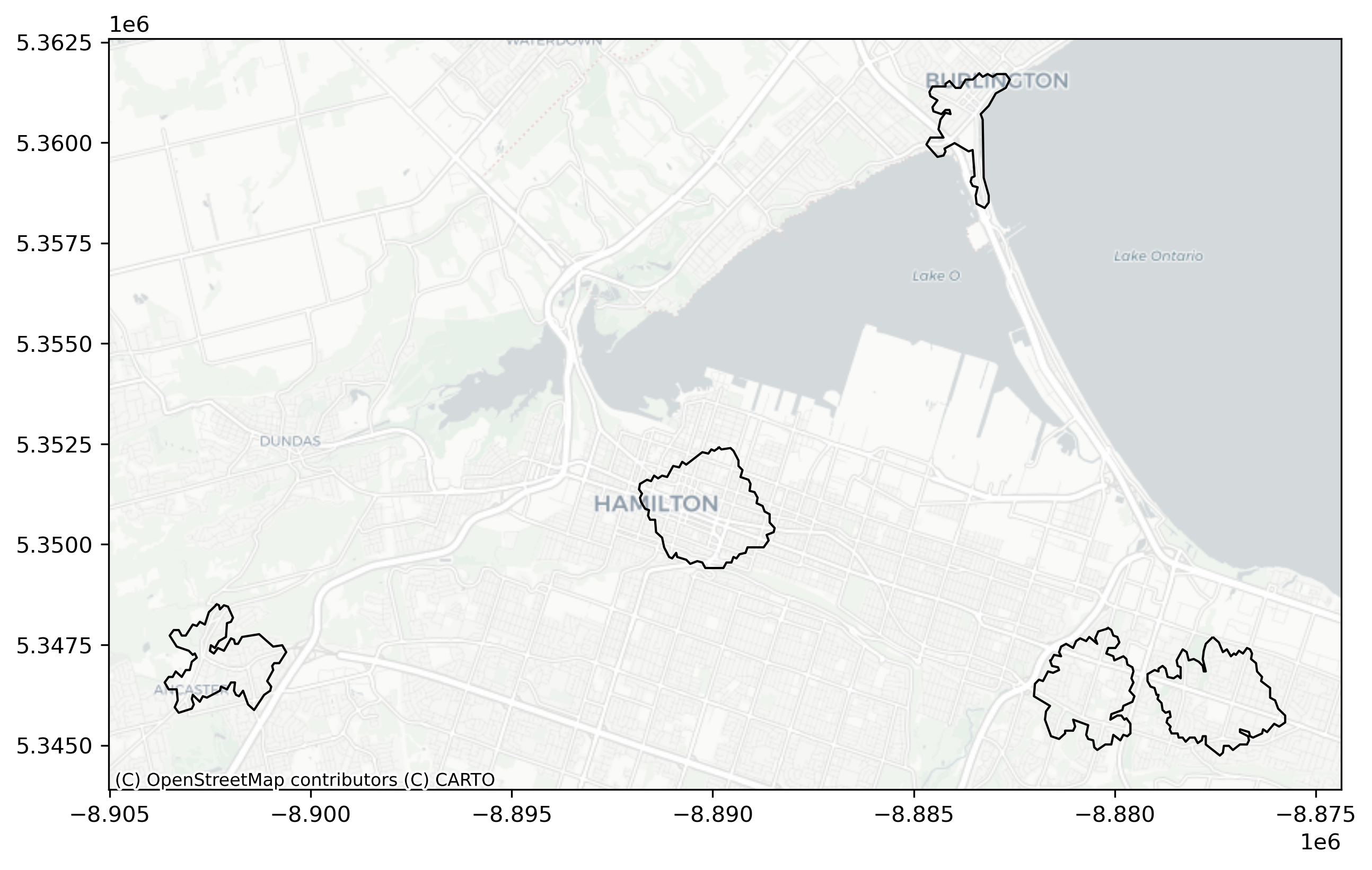
By following these steps, you’ll be able to compute catchment areas for transit stops programmatically. The resulting data can be utilized for further analyses, such as evaluating accessibility and coverage of public transportation networks.