
Evaluating vegetation change in Wolf Creek, YT with multi-temporal LiDAR: Part 1
In this post, I’ll be giving a summary of my current MSc progress in the McMaster Watershed Hydrology Group. This thesis project has two main components: using LiDAR and other remotely sensed imagery to quantify vegetation change over time in a subarctic research watershed, and comparing how these changes vary over different landscape properties. This first post focuses on how I created shrub cover layers by combining field surveys and remotely sensed data, while Part 2 will elaborate on these results and how to show how vegetation change is occurring preferentially in areas with specific topographic characteristics.
Introduction
High-latitude ecosystems have experienced substantial warming over the past 40 years [1, 2, 3], causing an increase in vegetation growth throughout the circumpolar North [4, 5]. A major component of this change is shrub expansion in arctic and subarctic ecotones [5, 6]. The rates of shrub expansion are highly variable depending on plant species, topographic position, hydrology, soils, and other ecosystem properties [6]. Changes in shrub and other vegetation properties are critical to document due to their first-order control on water, energy, and carbon balances [5]. Understanding these changes is critical for predicting the future of northern watersheds under a rapidly changing climate. This study uses multi-temporal airborne LiDAR, optical imagery, and field surveys to quantify shrub expansion over 11 years in a well-studied subarctic mountain basin.

Study Area
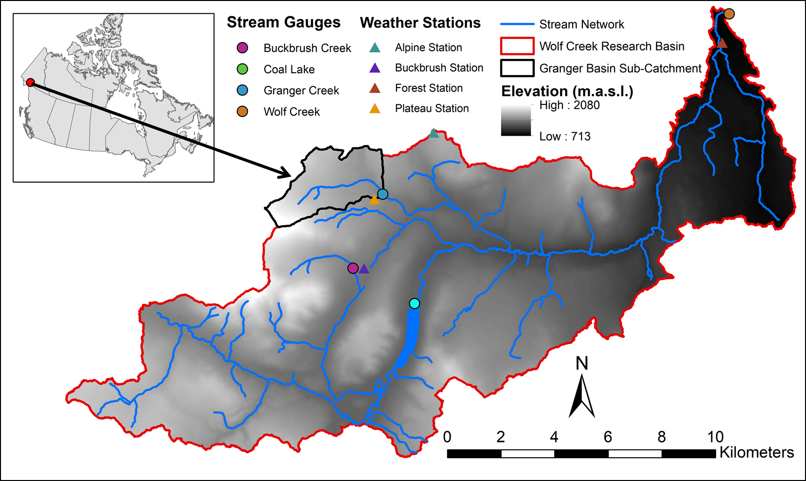
This study was conducted in the Granger Basin, a ~7.6km2 subarctic headwater catchment located in the Wolf Creek Research Basin (WCRB) [7]. The WCRB is a long-term watershed research facility located ~15km south of Whitehorse, Yukon Territory [8]. Granger Basin straddles the WCRB’s subalpine and alpine tundra ecozones, with an elevation range of 1356 to 2080 m.a.s.l. and a subarctic-continental climate [9]. While both the overall WCRB and Granger Basin have over 20 years of comprehensive meteorological data on record [10], there remains a lack of research on its vegetation and its influence on the hydrological cycle.
Field Methodology
In order to find out how well LiDAR can model vegetation, we need to first get boots on the ground to figure out what’s actually there. For the field campaign of this project, 29 vegetation transects were spread throughout Granger Basin to evaluate shrub properties for comparisons to the LiDAR.
Target sites were navigated to in the field using the Collector for ArcGIS mobile application. Each 40m transect consisted of 5 circular plots with a 1m radius, spaced out at every 10m (Figure 3). Field measurements were appended to differential GPS coordinates of plot centroids in R Statistics and used to create new plot area shapefiles through the R-ArcGIS Bridge and ArcPy scripting.
LiDAR Processing
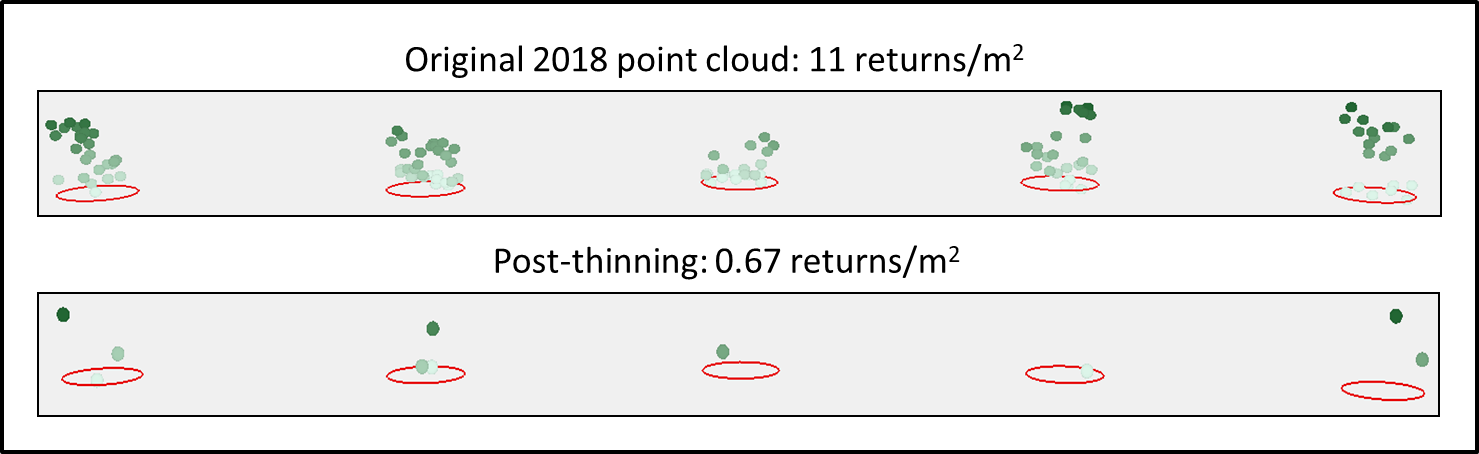
Airborne LiDAR surveys of the WCRB were conducted in August 2007 (return density = 0.67/ m2) and August 2018 (return density = 11.9/ m2). As lower sampling rates make LiDAR pulses more likely to miss the highest points of vegetation and underestimate heights compared to field measurements [11], these differences in survey resolutions had to be accounted for. The 2018 point cloud was thinned to an average density of 0.67/m2 to match with 2007 by randomly retaining a specified fraction of its original returns. Once all point clouds were pre-processed and height-normalized through LAStools batch scripting [12], height-above-ground (HAG) metrics were extracted for each plot radius (Figure 5). These were compared to field measurements to evaluate how well the LiDAR surveys could estimate plot vegetation heights, with the goal of evaluating changes in height over time
The ability of the 2018 survey to model shrub presence and absence was also explored. Binary supervised classifications based on LiDAR metrics were conducted through the Random Forests (RF) and Support Vector Machines (SVM) machine learning classifiers in R Statistics, using field data for model training and validation. 9 predictor variables derived from the LiDAR were explored for use, which were then reduced to only 3 for the final classifications due to strong statistical relationships found using Spearman’s rank-order correlation coefficient. 25 iterations per classifier were conducted using a loop with different random seeds to explore the effects of training/validation set selection on classification accuracy and class stability.

The classification model producing the best overall independent accuracy and class stability over different iterations using the thinned 2018 point cloud was applied to the 2007 LiDAR survey to create raster layers representing shrub cover in Granger Basin for both years. By subtracting the 2007 layer from 2018, a new change layer was created where pixel values of 1 = shrub growth, 0 = no change, and -1 = shrub loss. Layers representing stable shrub and stable non-shrub pixels were also created from pixels with identical values of 1 and 0 respectively in both classifications.
Results
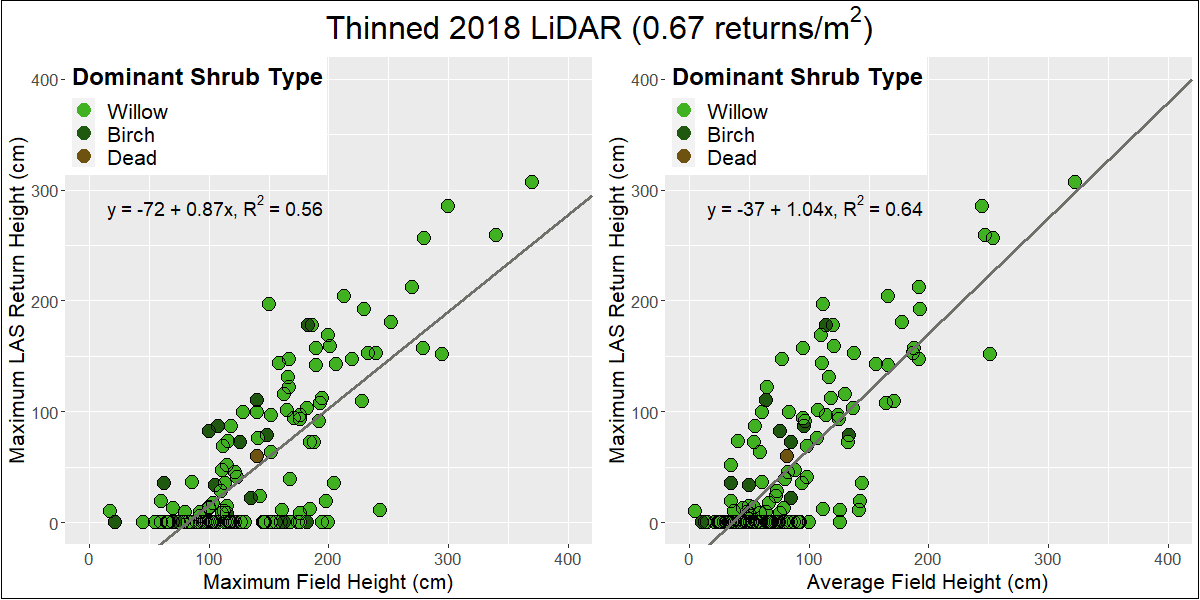
The original high-density 2018 point cloud was found to underestimate maximum field-measured heights within the 1m plots by only 11cm on average, with an overall R2 of 0.79 (Figure 6). However, we can’t compare these to 2007 before thinning due to the influence of higher return densities on height estimation.

Thinning the point cloud substantially decreased accuracy across the board, most likely from increased sampling error as a result of its lower return density.
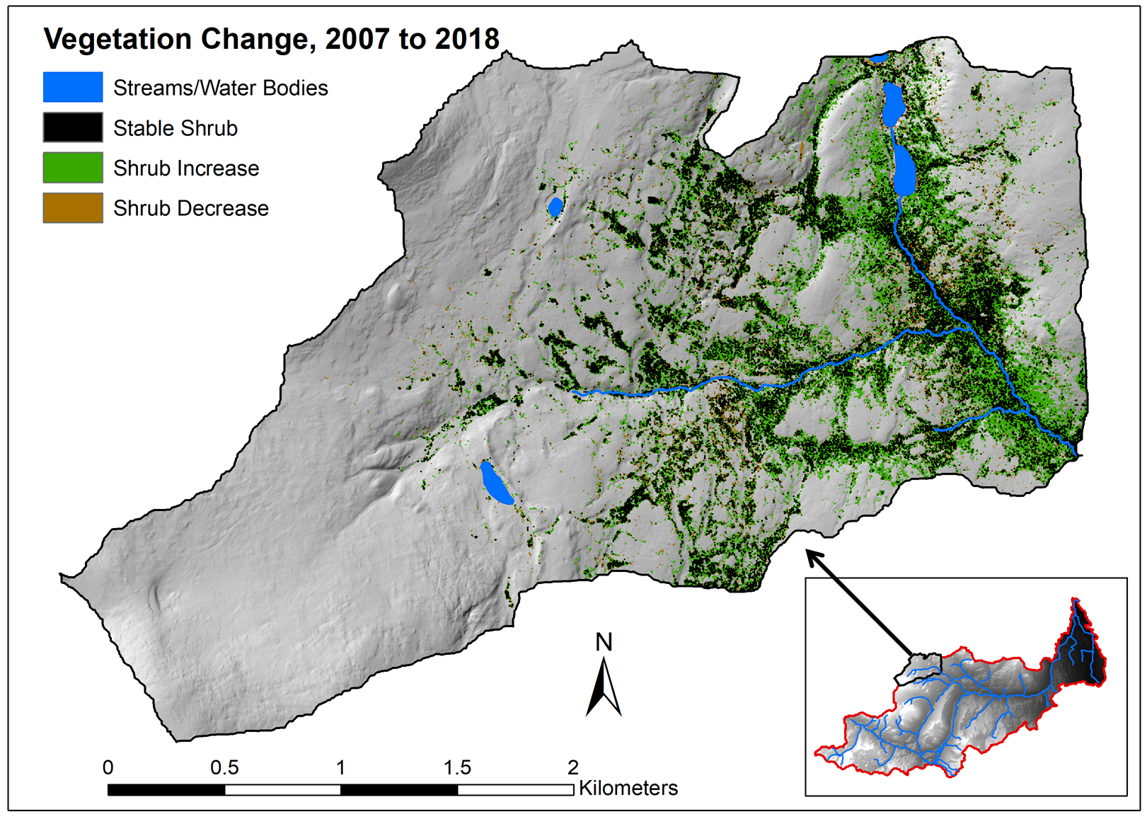
Due to these high levels of height underestimation, binary presence and absence models for the thinned 2018 LiDAR were used instead to evaluate change over survey years. After consolidating error matrices over the random seed iterations, RF gave a higher average accuracy, kappa coefficient, and more stable class areas and was therefore chosen over SVM for the final classifications. The best-performing RF classification with 97.1% overall independent accuracy gave 1.60km2 of shrubbed area in 2018 compared to 0.98km2 when applied to 2007. The change layer created by subtracting the 2007 shrub cover layer from 2018 (Figure 8) shows clear and substantial increases in shrub cover throughout the lower basin, with a 64% increase in total shrub area between the LiDAR surveys.
Conclusion
Airborne LiDAR was used along with field surveys to evaluate changes in vegetation cover over time in a well-studied subarctic mountain basin, with results showing clear and substantial increases throughout the study area between 2007 and 2018. However, just quantifying shrub expansion within the basin isn’t enough as the rates of this phenomenon are known to be highly variable within individual study areas. Upon a visual inspection we can see that both stable and expanding shrub pixels appear to be predominantly located in areas close to the interconnected stream network and at lower topographic positions. For my next post, I’ll be moving on to statistically comparing how these changes vary over the basin according to terrain properties such as slope position, aspect, topographic wetness, and more. Stay tuned!
Work Cited
- Hinzman, L. D., Bettez, N. D., Bolton, W. R., Chapin, F. S., Dyurgerov, M. B., Fastie, C. L., … Yoshikawa, K. (2005). Evidence and implications of recent climate change in Northern Alaska and other Arctic regions. Climatic Change, 72(3), 251–298.
- Overpeck, J., Hughen, K., Hardy, D., Bradley, R., Case, R., Douglas, M., … Zielinski, G. (1997). Arctic environmental change of the last four centuries. Science, 278(5341), 1251–1256.
- Tape, K., Sturm, M., & Racine, C. (2006). The evidence for shrub expansion in Northern Alaska and the Pan-Arctic. Global Change Biology, 1(2), 686–702.
- Myers-Smith, I. H., Forbes, B. C., Wilmking, M., Hallinger, M., Lantz, T., Blok, D., … Hik, D. S. (2011). Shrub expansion in tundra ecosystems: Dynamics, impacts and research priorities. Environmental Research Letters, 6(4).
- Epstein, H. E., Myers-Smith, I., & Walker, D. A. (2013). Recent dynamics of arctic and sub-arctic vegetation. Environmental Research Letters, 8(1).
- Tape, K. D., Hallinger, M., Welker, J. M., & Ruess, R. W. (2012). Landscape Heterogeneity of Shrub Expansion in Arctic Alaska. Ecosystems, 15(5), 711–724.
- Carey, S. K., Boucher, J. L., & Duarte, C. M. (2013). Inferring groundwater contributions and pathways to streamflow during snowmelt over multiple years in a discontinuous permafrost subarctic environment (Yukon, Canada). Hydrogeology Journal, 21(1), 67–77.
- Janowicz, J. R. (1999). Wolf Creek Research Basin – Overview. Department of Indian and Northern Affairs Canada.
- McCartney, S. E., Carey, S. K., & Pomeroy, J. W. (2006). Intra-basin variability of snowmelt water balance calculations in a subarctic catchment. Hydrological Processes, 20(4), 1001–1016.
- Rasouli, K., Pomeroy, J. W., Janowicz, J. R., Williams, T. J., and Carey, S. K. (2019). A long-term hydrometeorological dataset (1993– 2014) of a northern mountain basin: Wolf Creek Research Basin, Yukon Territory, Canada. Earth System Science Data, 11, 89–100.
- Zhao, K., Suarez, J. C., Garcia, M., Hu, T., Wang, C., & Londo, A. (2018). Utility of multitemporal lidar for forest and carbon monitoring: Tree growth, biomass dynamics, and carbon flux. Remote Sensing of Environment, 204(September 2016), 883–897.
- Isenburg, M. (2019). LAStools – efficient tools for LiDAR processing. Version 190927, http://lastools.org