
Integrating GIS and Field Work in Wolf Creek, Yukon Territory
I’ve spent the past summer working as a research assistant for my M.Sc supervisor Dr. Sean Carey, before officially starting grad school in September. Through helping out the other grad students in our lab, I’ve learned tons of valuable hydrology-specific GIS skills (which I could write about in a future blog post), but I want to focus here on some of the work I will be doing as a grad student over the next two years.
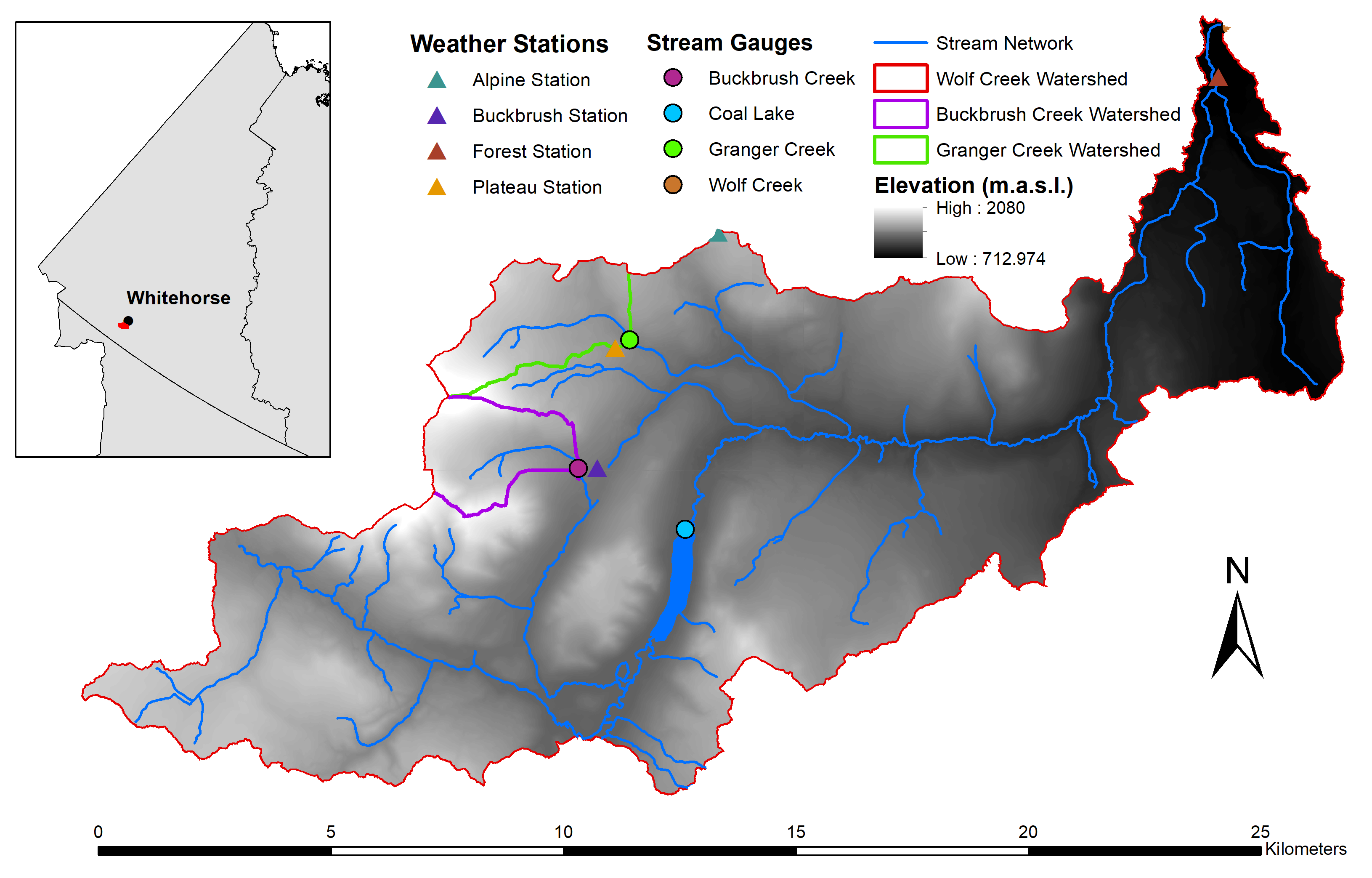
Though the full extent of my M.Sc project hasn’t been finalized yet, an important component will be reclassifying the Wolf Creek Research Basin (WCRB). The WCRB is a ~180km2 hydrologic basin located about 20km south of Whitehorse, in the south-central Yukon Territory (Janowicz, 1995). My supervisor Dr. Carey has been studying the WCRB for over 20 years, with much of that work being through our McMaster Watershed Hydrology Group.
The previous ecological classification of the basin was done all the way back in 1997, using GRASS GIS and four primary spatial data sources: a supervised classification of Landsat 5 TM imagery, a detailed vegetation inventory, a 30m DEM, and high-quality air photos (Francis, 1997).
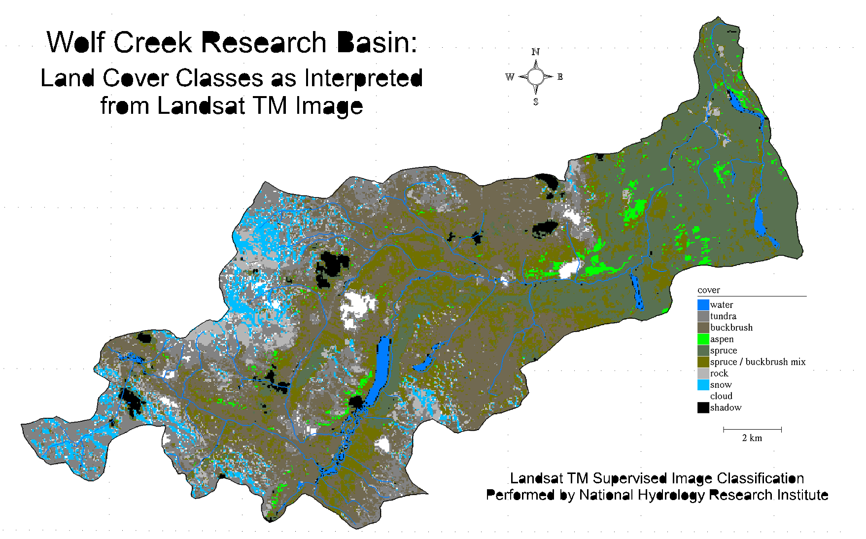
A supervised classification is only the first step in a full ecological classification, no matter what the quality. For example, even high-quality remotely sensed imagery encounters problems differentiating tree and/or shrub types with similar spectral signatures, such as boreal spruces and pines. There will also always be issues with clouds and shadow creating artificial spectral classes, as seen in the 1997 classification. The identification of wetland areas can also be problematic with spectral data, with the use of radar or thermal bands only being a partial fix.
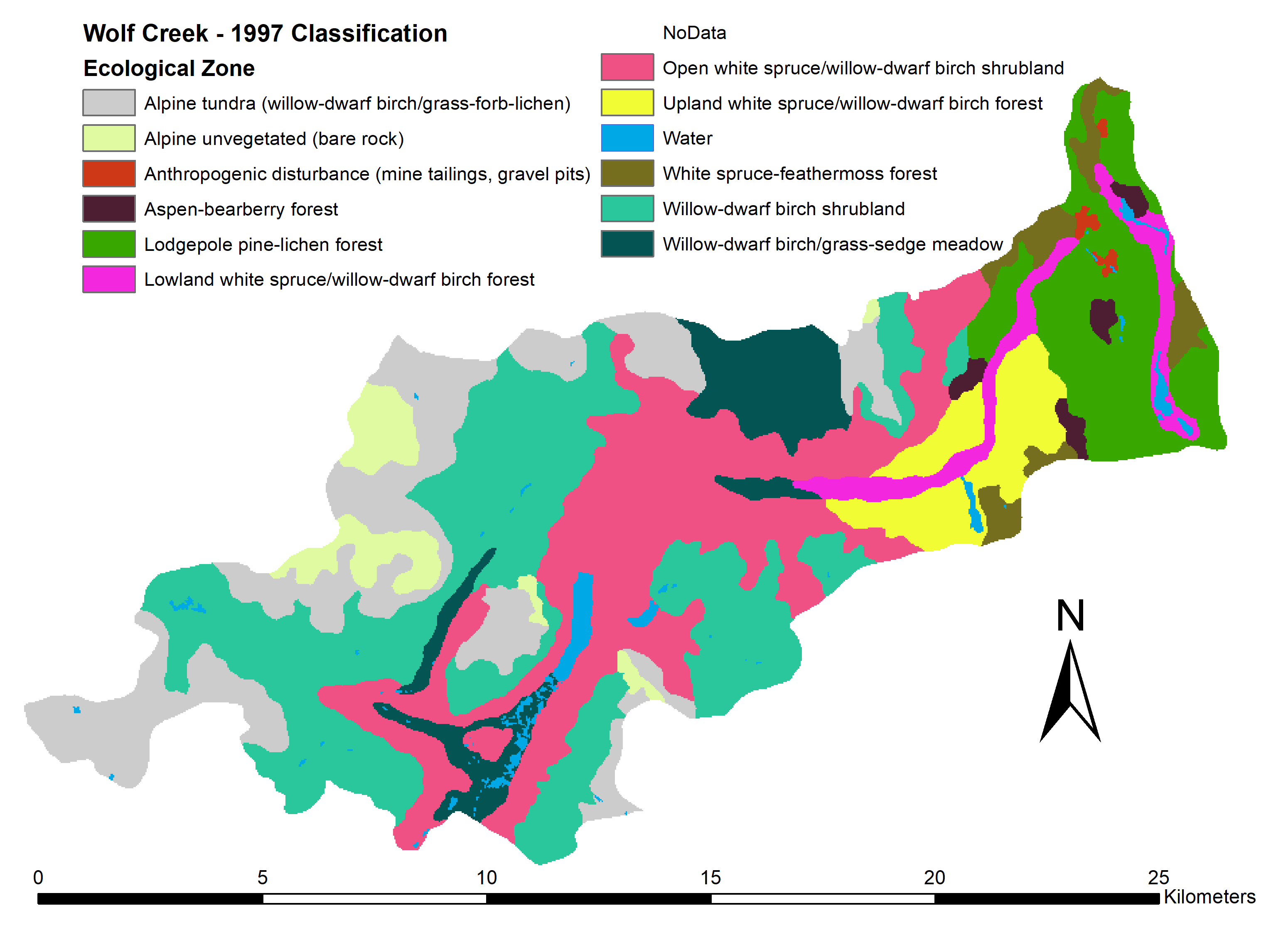
Due to these inherent limitations, the DEM was used to aid in boundary placement, creating three primary ecozones based on an increasing elevation gradient: boreal, subalpine, and alpine. Vegetation inventory maps were used to identify specific ecologically meaningful communities within these zones, with the air photos as an aid. The final result of this process is as follows.
For our new classification of the basin, we will have some resources that did not exist in the same quality back in 1997. The Landsat 8 OLI is now operational, giving us higher-quality multispectral data to work with using ArcGIS Pro’s object-based supervised classification. There are also even higher resolution commercial satellites out there, if we choose to go that route in the future. Even with this level of improvement in imagery and classification software, field measures and a more accurate DEM will be needed to supplement this.
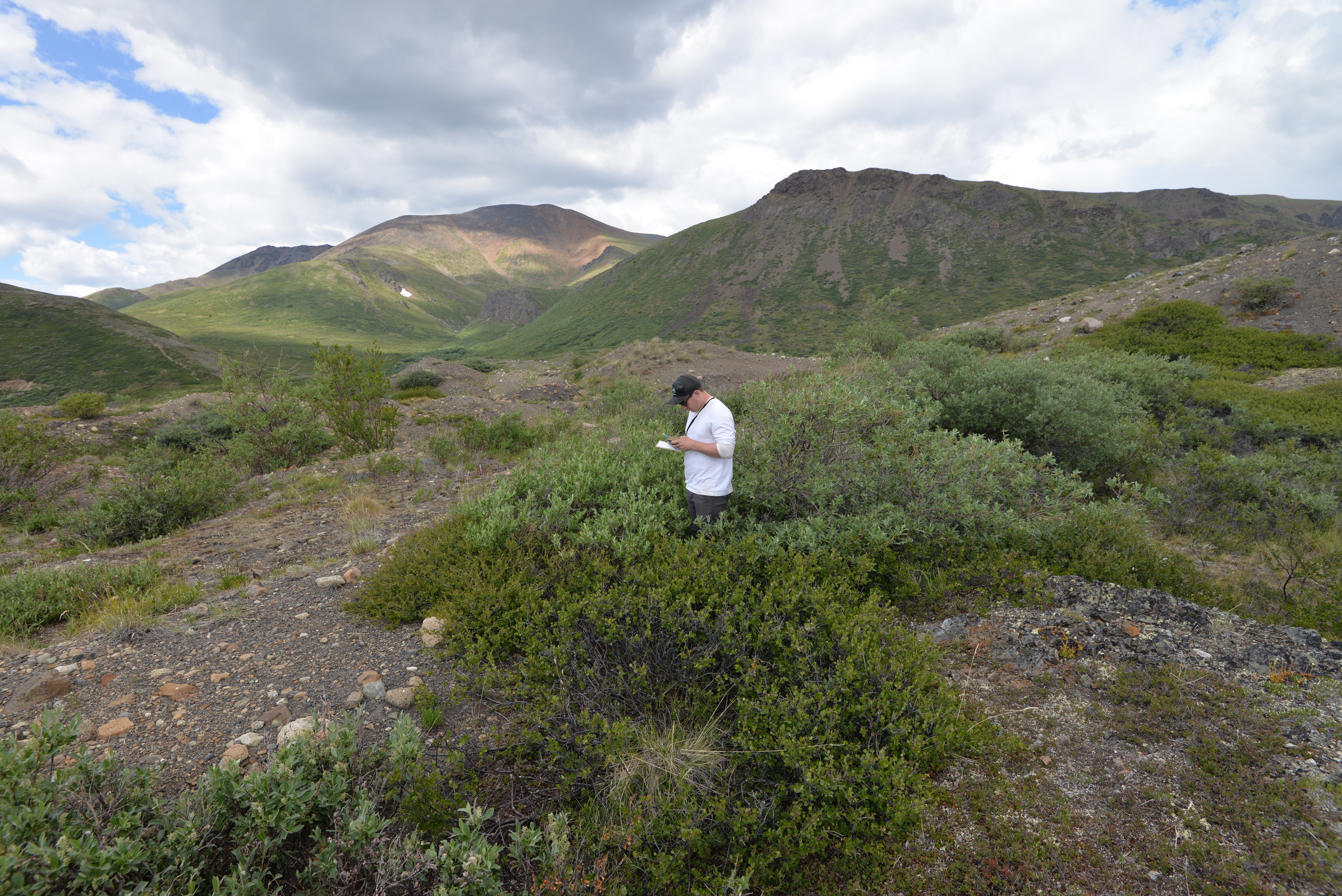
Though my official field season won’t start until next summer, I spent some time in Whitehorse with the crew in July getting acquainted with the research site and helping out our lab’s other grad students with their work. Getting to see the basin in person after only working with spatial data in ArcGIS for two months was amazing, and helped me realize the amount of work and preparation needed to have a successful field season. A big part of my time there was spent figuring out the logistics behind which ground truthing information would be most important for this project, and where these points might be best located. I was able to get lots of advice from our field techs up there on what areas within the basin haven’t been as explored, and run ideas by them of what field work might be best for my project.
Another idea that we’ve been looking into is estimating vegetation density through differences in Lidar returns (i.e. 1st returns as a DSM vs. ground returns as a DEM), and comparing this to vegetation height transects taken in the field. Preliminary work for this has been done using the LAStools software suite, which has a great range of functions that can be used through either the command line, a GUI, or pre-packaged into ArcGIS Toolboxes. A helpful addition to these is their Production Toolbox, which allows for batch processing of multiple datasets through all their existing functions without having to write additional Python scripts to loop over them. Though there are some boundary issues with the Lidar we have right now, our proof-of-concept type work is looking promising enough to apply to new datasets once they become operational.
There is still a huge amount of work to be done towards designing a field program for next summer: how to design our ground truthing network, how closely to follow the 1997 classification’s ecozones, which areas are lacking in coverage, and more. I’m excited to work out all these logistics, get back in the field, and see what we can do with this wealth of data over the next two years.
Work Cited:
Francis, S. 1997. Data Integration and Ecological Stratification of Wolf Creek Watershed, South-Central Yukon. Applied Ecosystem Management Ltd.
Janowicz, J.R. 1995. Wolf Creek Research Basin, Yukon. Department of Indian and Northern Affairs Canada.