
Delineating Urban Lake Watersheds using Arc Hydro
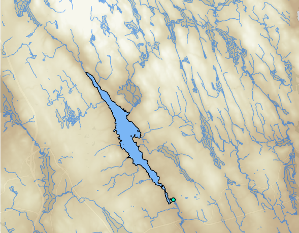
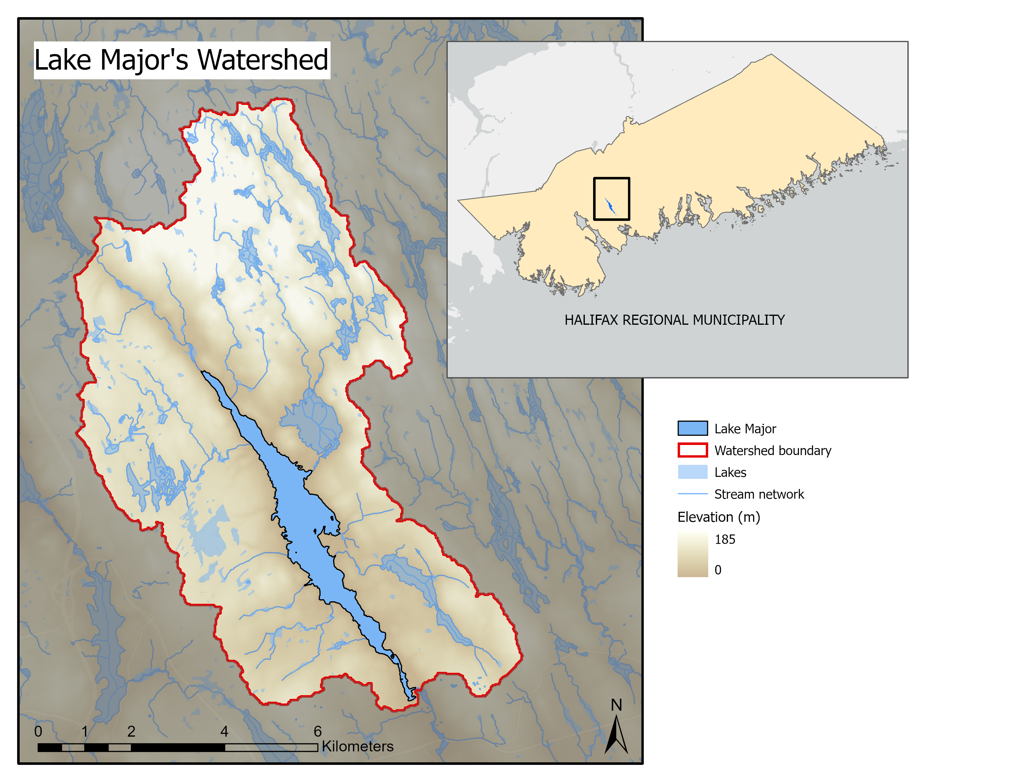
Many natural and anthropogenic processes occurring within a lake’s watershed directly affect lake water quality (Soranno et al., 2015). As such, delineating the bounds of a lake’s watershed is often the first step towards identifying factors driving changes in water quality over time. This critical step can be achieved with the help of Arc Hydro, which provides a data model, a toolset, and workflows directly pertaining to water resources applications (Esri, 2019). The workflow below details the steps executed in my research, that focuses on changes in water quality across a 40-year period within a set of Halifax-area lakes in Nova Scotia. The delineation process for Lake Major (Fig. 1) is illustrated throughout this piece.
Inputs and Data Preparation
The following data were required:
- Hydrologically conditioned digital elevation model (DEM)
- Stream network
- Lake outfall locations
An enhanced 20m DEM for the province was accessed from the Nova Scotia Department of Natural Resources and Renewables website, and the Provincial Hydrographic Network (containing the stream network) was accessed from Nova Scotia’s Geographic Data Directory. Lake outfall locations were determined by viewing lake bathymetry maps and cross checking with the National Hydrographic Network, whenever possible, and were marked with a “Pour Point” (Fig. 1).
To improve processing speeds, both the stream layer and DEM were subset to an area several times larger than the anticipated size of the watershed. Additionally, all layers were projected to the same projected coordinate system as per the Arc Hydro Technical Guide (Esri, 2011).
Although the NS DEM asserts that it is “hydrologically correct,” the following preprocessing steps were taken to ensure it was hydrologically conditioned (i.e., it correctly models the flow of water across the surface) (Djokic, 2015).
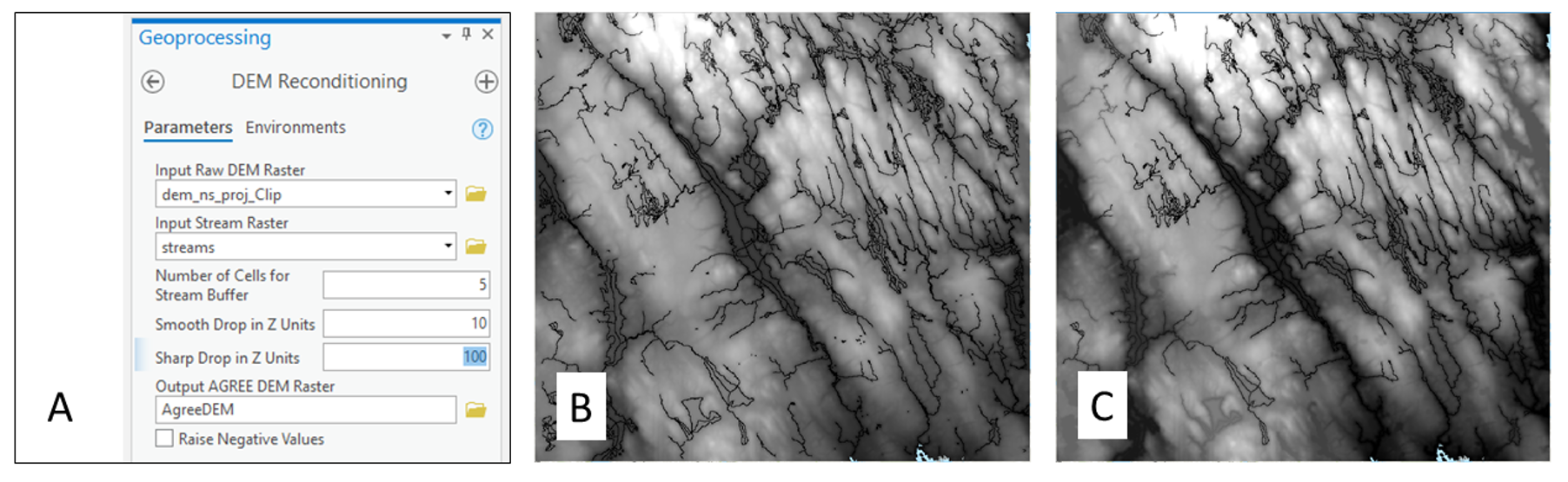
- DEM Reconditioning “burns” your stream network into your DEM and requires that you first convert your stream network into a raster (Fig. 2b). (Burning is the process of decreasing the elevation of a DEM along a linear feature to enforce the proper drainage across the surface). The tool allows the user to manipulate the “buffer,” which is the horizontal distance in cells away from the stream, the “smooth drop,” which is the vertical drop at each unit of the buffer, and the “sharp drop,” which is the vertical depth of the line itself (Fig. 2a).
- The Fill Sinks tool identifies cells having values lower than their surrounding cells and are often errors that result from the resolution of the dataset (Esri, n.d.). The tool aims to correct these cell values as their presence in the surface can interrupt the derived drainage network (Esri, n.d.) (output shown in Fig. 2c).
Terrain Processing
- Once a hydrologically conditioned DEM has been obtained, the Flow Direction tool can be applied. This tool scans the elevation of each cell to identify the direction of steepest decent and assigns values to the output raster which indicate which neighboring cell water would flow into (Fig. 3a).
- The Flow Direction output can then subsequently be used by the Flow Accumulation tool to create a raster output where each cell contains the value of upstream cells draining into the focal cell (Fig. 3b). The stream network is easily distinguishable in the output, and the directionality becomes clear as well since the values increase as you move farther downstream (Fig. 3b).
- This Flow Accumulation output can then be used by the Stream Definition tool, to produce a new stream raster where only cells that receive enough flow from upstream cells are recognized; all other cells that are not recognized by the process are assigned as “No Data” cells (Fig. 3c). This intermediate step is intended to speed up point delineation and, therefore, the output does not need to match the original stream network (Esri, 2011). The recommended threshold for stream determination is 1% of the maximum flow accumulation and appears as the default number of cells that will define a stream (Esri, 2011). Selecting too small of a threshold will create a denser stream network which could negatively impact delineation performance (Esri, 2011).

Sub-catchment polygons were generated over the following three steps (Fig. 4).
- First, the new stream raster is divided into individual stream segments with the help of the Flow Direction raster by the Stream Segmentation tool (Fig. 4a).
- The Catchment Grid Delineation tool then identifies the area draining into each stream segment (again, with the help of the Flow Direction raster) and assigns a unique value to the cells within each sub-catchment, as shown in Figure 4b.
- Finally, this raster is converted to a polygon layer through the Catchment Polygon Processing tool (Fig. 4c).

- Returning to the output from the Stream Segmentation tool, the Drain Line Processing tool converts the raster to a vector line layer (Fig. 5a). This step also assigns information to each feature regarding connections to downstream features and the catchment it belongs within.
- The Adjoint Catchment tool aggregates sub-catchment polygons from the Catchment Polygon Processing output that drain to the same point based on the Drain Line Processing output and stores them in a new polygon feature layer (Fig. 5b). This step aims to speed up the point delineation process.
- The Drain Point Processing tool also makes use of the Catchment Polygon Processing output, as well as the Flow Accumulation output (which had not been used up to this point). A new point feature layer is created, and points are placed at the lowest (farthest downstream) point of each sub-catchment (Fig. 6a).
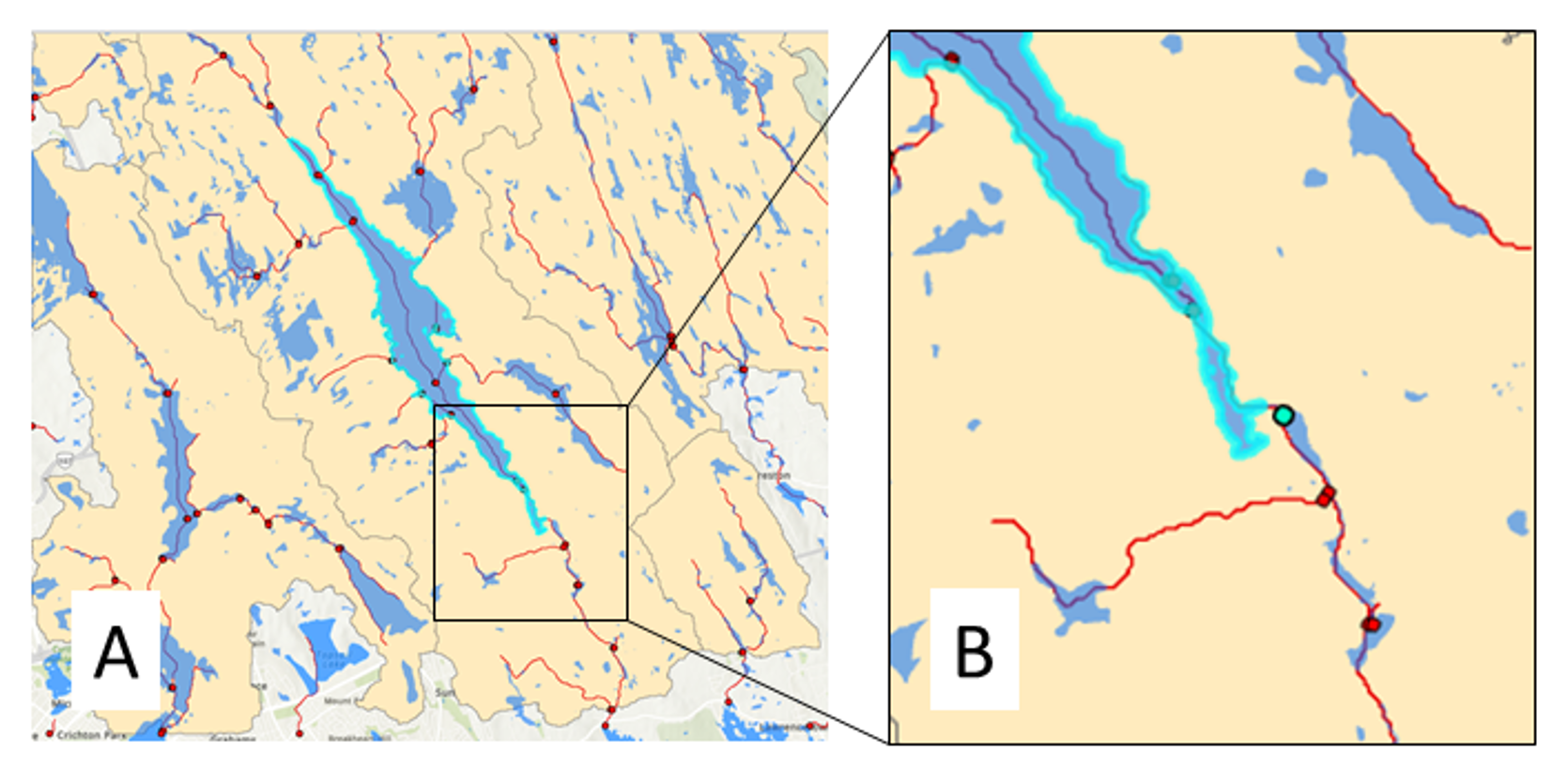
- Finally, the Point Delineation tool creates a polygon indicating the bounds of the watershed, based on the location of the Pour Point. The resulting watershed delineation for Lake Major is depicted in Figure 7.
Due to the urban nature of many of the lakes within this dataset, manual adjustments were often required to account for storm water infrastructure, which interrupts the natural flow of water across the landscape. The watersheds derived from this workflow will be used to quantify watershed characteristics such as road densities which may, in turn, reveal connections between changes in lake water quality and the natural and anthropogenic processes within each watershed.
References
Djokic, Dean. (2015). Creating a Hydrologically Conditioned DEM. Esri User Conference. Technical Workshop. Retrieved from: https://proceedings.esri.com/library/userconf/proc15/tech-workshops.html.
Esri. (2019). Arc Hydro: Project Development Best Practices. An Esri White Paper. Retrieved from: https://www.esri.com/en-us/industries/water-resources/arc-hydro.
Esri. (2011). Arc Hydro Tools – Tutorial. Version 2.0 – October 2011. Retrieved from: https://downloads.esri.com/archydro/archydro/tutorial/doc/.
Esri. (n.d.). How Fill Works. Retrieved from: https://pro.arcgis.com/en/pro-app/2.8/tool-reference/spatial-analyst/how-fill-works.htm.
Soranno, P. A., Cheruvelil, K. S., Wagner, T., Webster, K. E., & Bremigan, M. T. (2015). Effects of land use on lake nutrients: the importance of scale, hydrologic connectivity, and region. PloS one, 10(8), e0135454.