Are you ready to be blown away by the magnificent mountains of Whistler, British Columbia? Whistler is not only famous for its stunning landscape and outdoor activities but also for being an excellent site for analyzing spatial relationships. In this blog post, we will delve into the importance of visibility and distance analysis in mountainous regions. We will explore the different techniques involved, such as linear and radial line of sight, cumulative viewshed, and distance allocation. These techniques help us identify visible areas, efficient routes, and appropriate locations for essential facilities such as fire stations, hospitals, and other public services. So let’s take a closer look at how these techniques can be used to analyze spatial data in Whistler, BC.

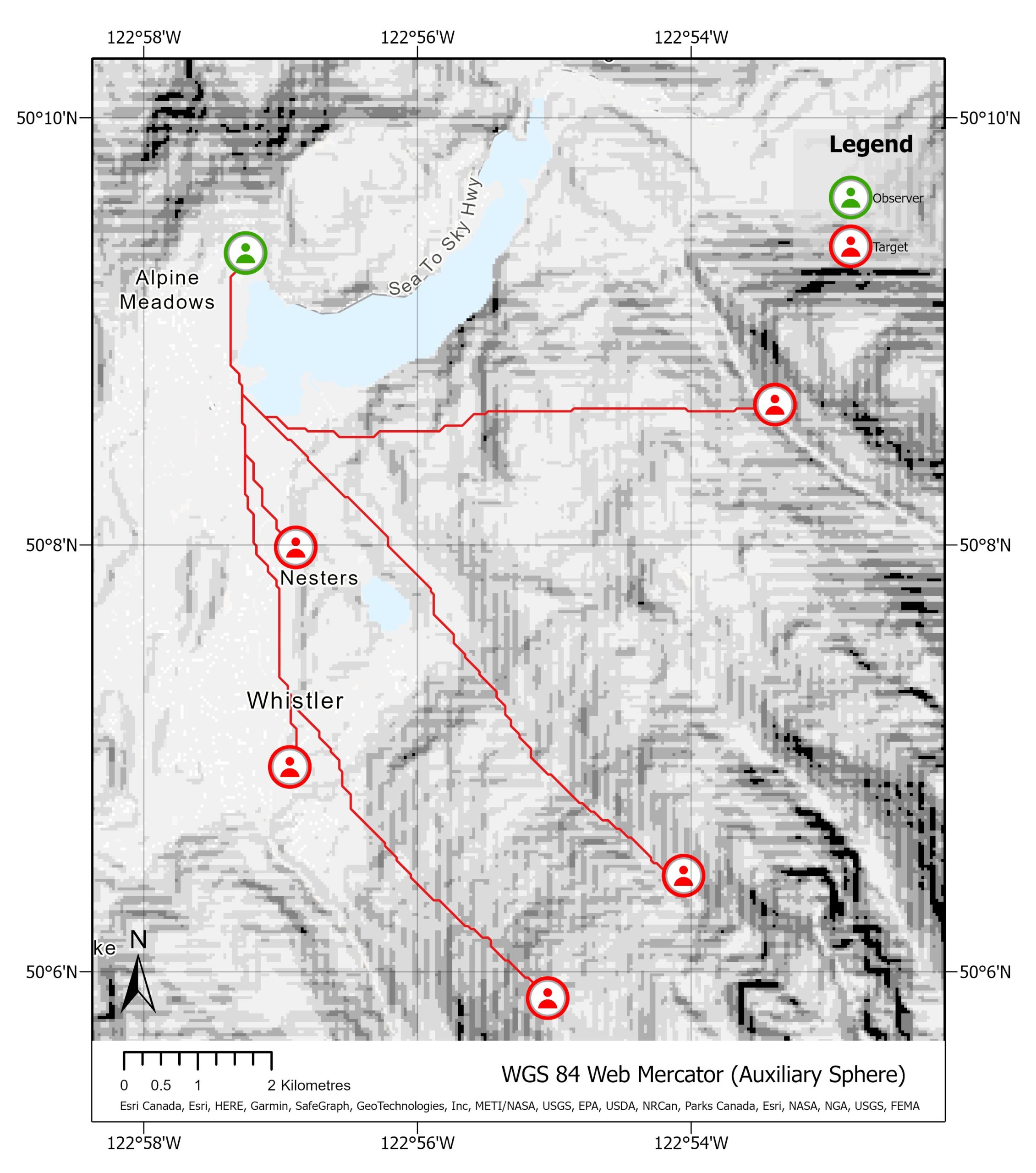
Study Area

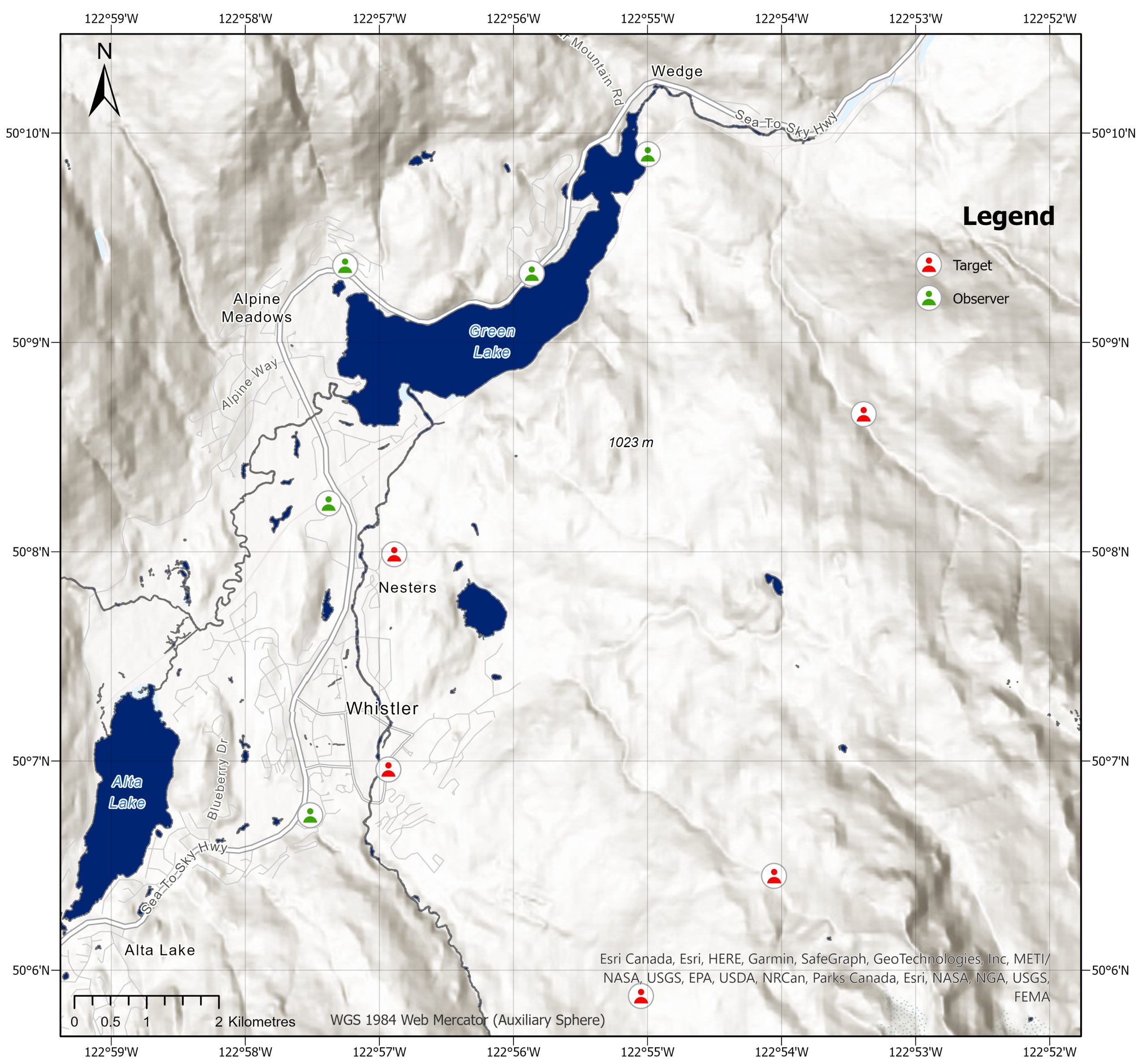
Behold the charming town of Whistler, where the magnificent mountains will astound you in every sense – from the stunning views to the fresh mountain air that will leave you breathless. But these mountains are not just a treat for the eyes; they also provide an excellent opportunity for analyzing spatial data. In this blog post, we’re going to play a little game of hide and seek with our five observers and five targets. Can our observers spot the targets from their vantage points, or will the targets remain hidden? Let’s find out using the power of visibility and distance analysis!

Visibility Analysis

Linear line of sight (LLOS)

Picture yourself as a spy on a mission, trying to figure out the best vantage point to keep an eye on your target. That’s where the line of sight comes into play! It’s like an imaginary laser beam connecting you and your target, helping you identify the areas that are visible and those that are out of sight. Whether you’re on a lookout tower or just standing on a mountaintop, understanding the line of sight is crucial for a successful mission. And remember, just like in spy movies, sometimes the valleys and areas behind mountains can be your best hiding spots!

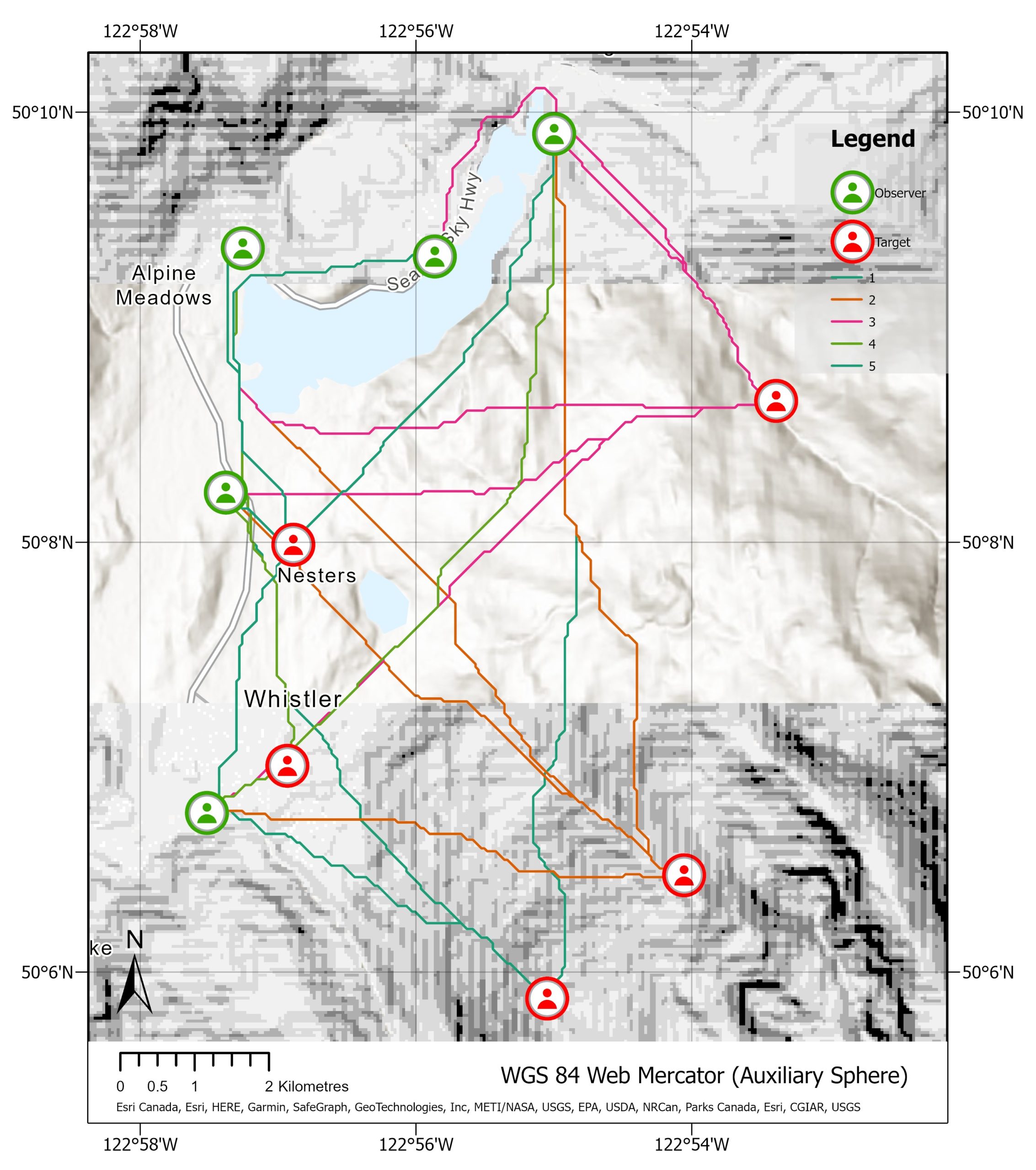
Required inputs: DEM, observer and target layers.

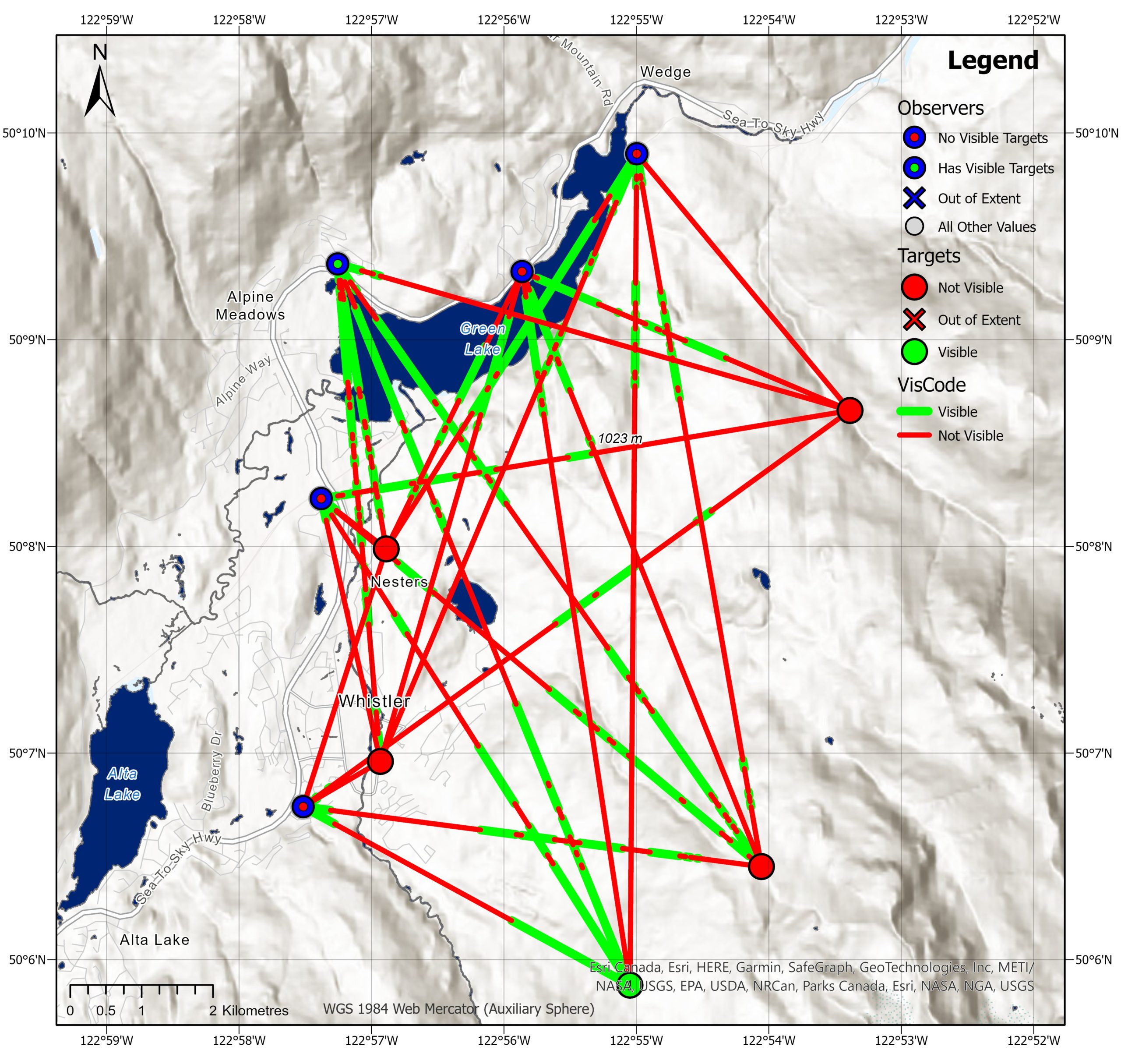
This visualization represents a map where lines are drawn from observers to targets. The height of the observers and targets are set to 2 metres. The green segments of the lines represent the visible areas, while the red segments indicate the non-visible areas. A red dot is placed inside an observer if there are no visible targets, whereas a green dot signifies that at least one target is visible. Based on this map, it appears that only one target is currently visible by one observer. This is due to the target being high up a mountain. The two observers to the south are able to see the area surrounding the target, but they do not have a clear line of sight to the target itself.

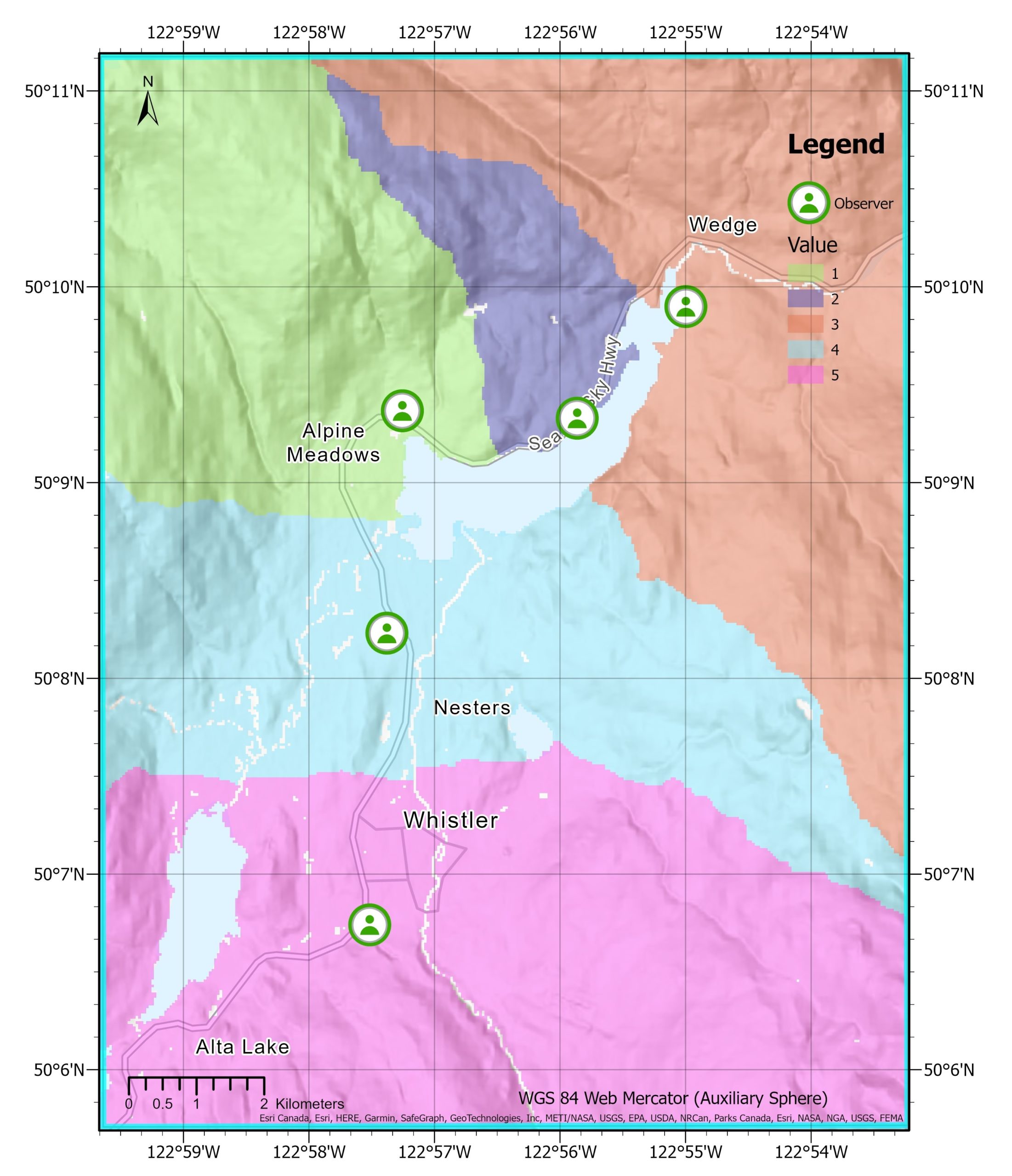
Radial Line of Sight (RLOS)

Get ready to put on your hiking boots because we’re about to explore the fascinating topic of radial line of sight! It’s like the regular line of sight, but enhanced – instead of just drawing a straight line from the observer to the target, we trace a series of radial lines to see what’s visible from the observer’s location. This technique is especially handy in places where the landscape is steep or complex, like the awe-inspiring mountains of Whistler, British Columbia.

Required inputs: DEM and observer layer.

This output generates a binary raster that represents the radial line of sight for each observer, where 0 indicates that the pixel is not visible and 1 indicates that it is visible. These rasters are then merged, with the pixel value indicating the number of observers that have a line of sight to that particular pixel. The observed distance parameter is set to 5km. When looking at the mountains in Whistler, it’s easy to find them because they are visible and noticeable to the observer.

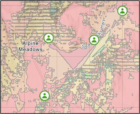
Here is a zoomed in image showing that there are some areas (in blue) seen by 4 observers. These are areas of high elevation relative to the observers.

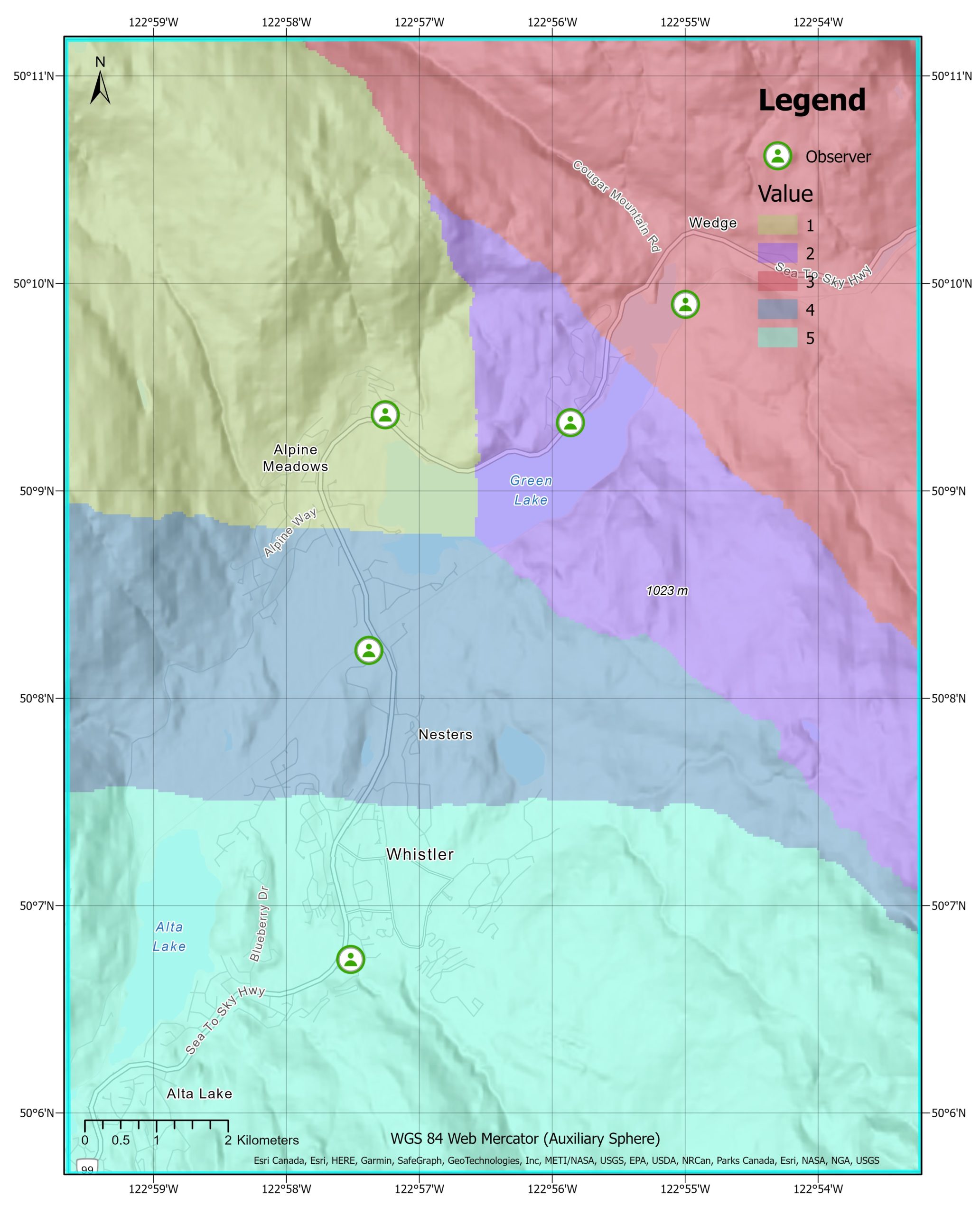
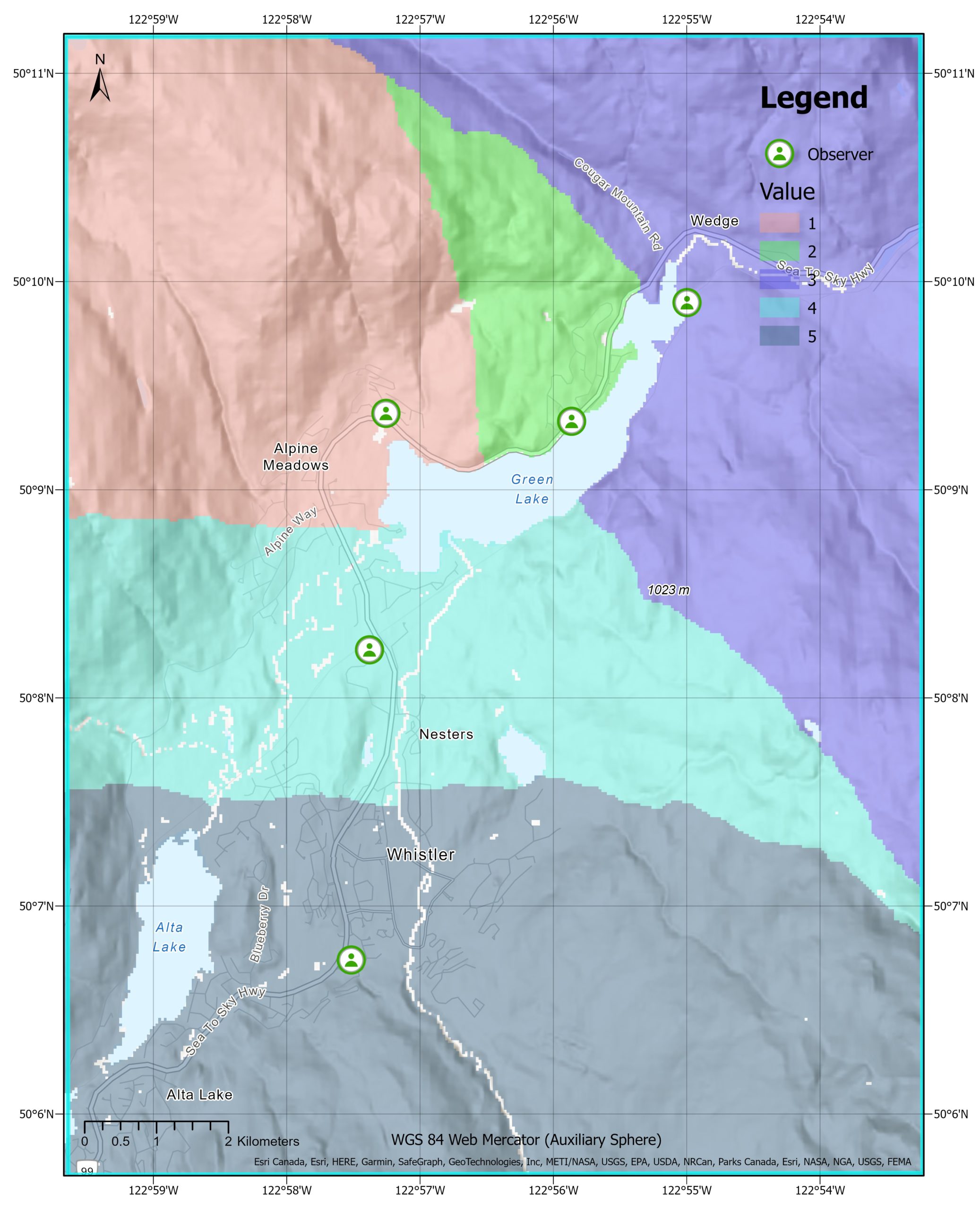
Cumulative Viewshed [Geodesic Viewshed (Spatial Analyst tools)]

A cumulative viewshed combines the visible areas from multiple observers, resulting in a comprehensive map of what can be seen from different vantage points. By merging individual viewsheds, decision-makers can identify areas of interest that may be affected by visibility, such as beautiful landscapes, fragile habitats, or key locations. So, next time you’re out in the field, don’t forget to create a cumulative viewshed and discover the hidden treasures of your environment!

Required inputs: DEM and observer layer.

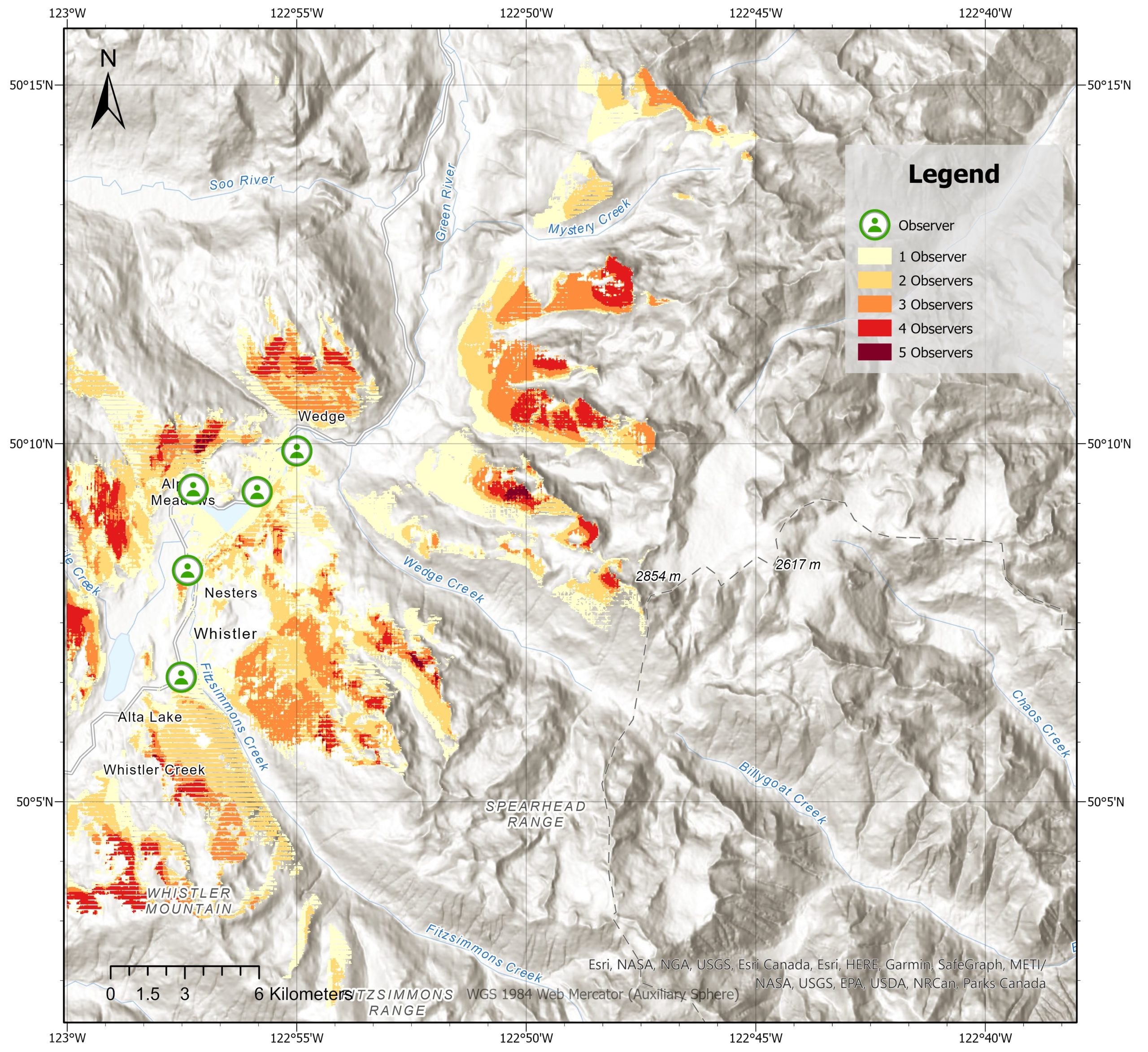
This is a cumulative viewshed with maximum distance of 20 kilometres showing a visual representation of the terrain and helps identify the areas that are visible and the areas that are obstructed by mountains or hills. As we can see, the 5 observers located in the valley are hindered by the towering mountains and hills surrounding them, limiting their visibility.

Distance Analysis

Distance Allocation

Distance allocation involves identifying the most efficient and cost-effective routes between an observer’s location and a target point. But not just straight-line distance! Barriers, surface distance and surface friction also come into play. It’s like a game of “choose your own adventure” for first responders trying to get to a fire or other emergencies in a hurry. But distance allocation isn’t just for emergencies – it’s also handy for figuring out where to put important public facilities like fire stations, hospitals, and paramedic bases.

Surfaces vary in their ease of traversal, and those that are simpler to traverse, such as dirt, should be prioritized and taken into consideration when allocating areas. Let’s not forget about slope – going uphill takes longer than a flat surface, so it’s important to assign the right person to the job. The person who arrives the fastest should be assigned to the area. And don’t forget about barriers like rivers or buildings – they’ll slow you down, so they need to be factored into the equation.

Required inputs: Cost Surface, barrier (optional), observers, and boundary.

Single-cost Surface

In a nutshell, single-cost surfaces are rasters that have cost values assigned to different areas. These could be land cover rasters, where certain areas like trees and swamps have a high cost assigned to them. Or they could be slope rasters, where each pixel is assigned a value indicating the steepness of the ground. This allows us to calculate the most efficient and cost-effective path between two points. Think of it like finding the shortest route on a map with varying terrains and obstacles! The path calculation involves analyzing the cost values of neighboring pixels and selecting the one with the lowest cost. It’s a powerful technique that’s widely used in fields such as transportation planning, emergency response, and environmental management.

For our single-cost surface, we are going to use the Slope tool on our DEM which will give each pixel a degree. Then we’ll use the Reclassify tool to assign the following values to the slope raster:

• Slopes ranging from 0 to 11: a value of 1
• Slopes ranging from 11 to 22: a value of 2
• Slopes ranging from 22 to 32: a value of 4
• Slopes ranging from 32 to 42: a value of 6
• Slopes ranging from 45 to 80: a value of 12

We’ll use the water bodies polygon layer as our barrier.

We will run the Distance Allocation tool twice, once with the slope raster as the cost surface and once with the barrier included as an additional factor to see the difference between the two.

The output on the left shows the distance allocation using the slope as a cost-surface. We see that the lines dividing each region aren’t perfectly straight which means the slope is affecting distances allocated.

As you can see on the image to the right, the water barrier has impacted the allocation of regions. The observer who was originally assigned to the purple region would now have to travel a longer distance around the lake, so the region has been reassigned to a nearby observer.

Weighted-cost Surface

The weighted cost surface is a useful tool in spatial analysis that models the cost of movement through geographic space. It achieves this by blending multiple single-cost surfaces with weights assigned based on their relative importance. The resulting composite surface provides a detailed view of the cost of movement across the landscape by accounting for variables such as terrain, slope, and land use. It’s a powerful and flexible tool widely used in GIS and remote sensing applications to identify optimal transportation routes, conservation areas, and more.

Ready to create your very own weighted cost surface? Here’s how it’s done: First, create a second single-cost surface by rasterizing the roads layer and giving roads a value of 1 and non-roads a value of 2. Next, using the Weighted Sum tool, blend this raster with the slope raster, where you can adjust the weights based on their relative importance. And voila, we have our weighted sum raster.

While the roads layer may not have been the most impactful variable, it nonetheless serves as an important example of the potential of distance allocation. So why not get creative and see what kind of weighted cost surface you can create?

Least Cost Paths

Have you ever wondered what the most efficient route is for your next hiking or biking adventure? Enter least cost paths! These efficient paths represent the most cost-effective routes between an observer’s location and a target point. It is important to note that least cost paths can be modeled in both directions – from observer to target and from target to observer – and may produce different results. It’s useful in analyzing the optimal routes for hiking, biking, or other outdoor activities. With the use of least cost paths, outdoor enthusiasts can plan their routes with greater efficiency and accuracy.

Required inputs: Cost surface, observer and target layers

By rasterizing the water bodies, this allows us to set the values as NoData and add them to the cost surface, resulting in a new cost surface with the barriers included. We’ll run the Least Cost Path tool twice, from each observer’s location to all target points, and from each target point to all observer locations.

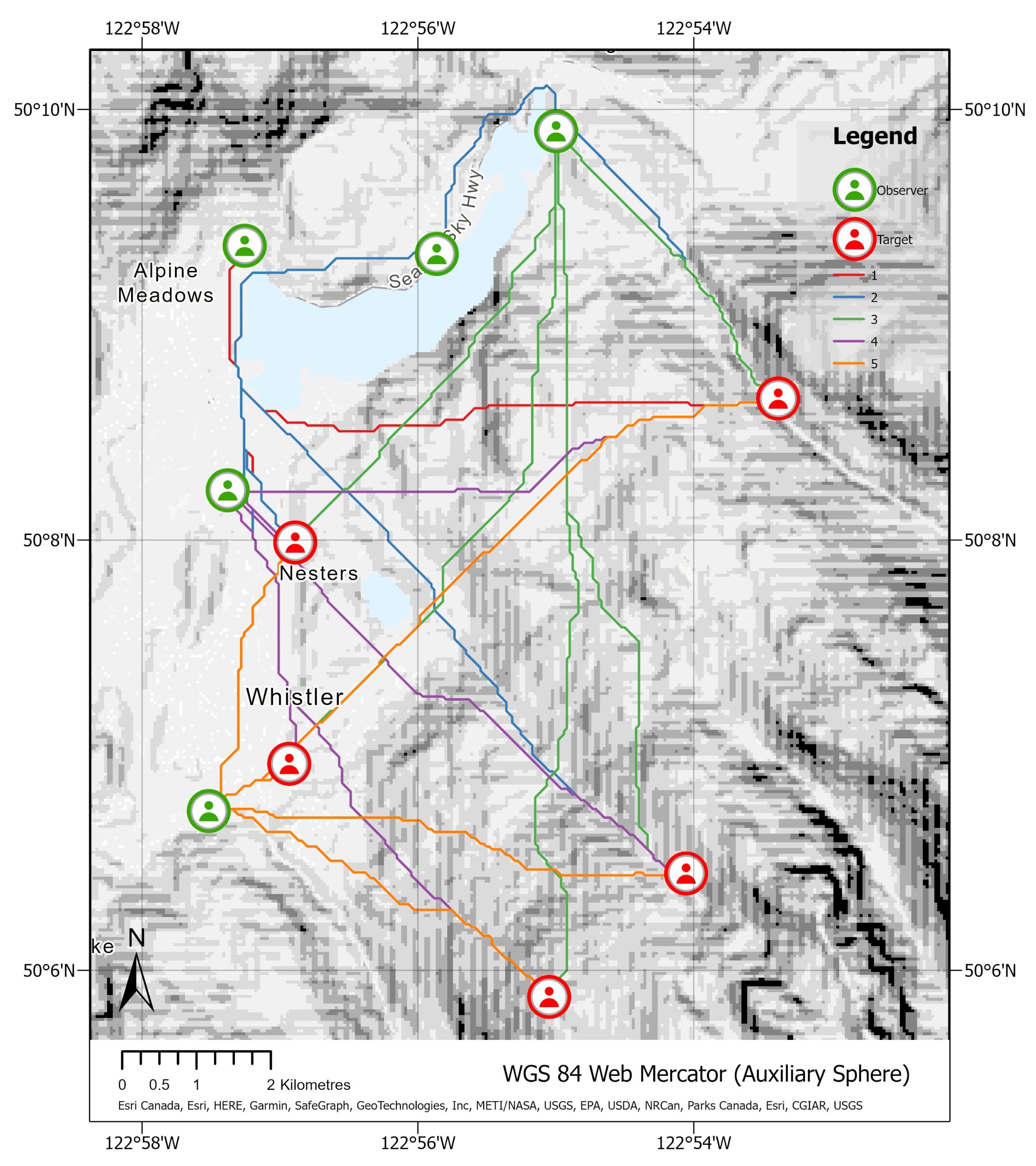
The image on the left showcases the output of the Least Cost Path tool applied from observers to targets, with the observer symbolization and the cost surface displayed. We can see that these paths are cleverly maneuvering around obstacles and taking the path of least resistance.

The image on the right showcases the Least Cost Path tool output when applied from targets to observers, symbolized by target. We can observe subtle differences in the most efficient path taken when compared to the opposite direction. This demonstrates that the straight-line Euclidean distance between points may not always be the most efficient route when we consider surface friction and obstacles.

This image provides a clearer view of the route taken from observer 1 to all the targets, including the path that leads up the mountains to the southeast. As our current cost surface considers only slope and roads, it does not incorporate land cover features such as forests and swamps. If we had access to such data, we could include it in our cost surface analysis for better accuracy. If you were curious about how far each path is, check out the attribute table – it’s got all the details on distances for all the paths.

Conclusion

In summary, ArcGIS Pro provides users with powerful tools for analyzing visibility and distance relationships, which can be applied in a wide range of fields such as urban planning, emergency management, and environmental management. With just a DEM and a point layer, users can easily perform visibility analysis, while distance analysis only requires a cost surface and a point layer. So, whether you’re trying to identify the best hiking trails, plan an optimal route for an emergency situation, or find the spot with the greatest views for a house, ArcGIS Pro can help you make more informed decisions and have fun while doing it!