
Python script to retrieve time-series changes in snow cover area from MODIS
As a part of Directed Studies in Geomatics course supervised by Dr. Murray Richardson at Carleton University I developed a tool that allows a user to easily produce time-series plots of snow-cover area and other relevant pieces of information (e.g. bare ground, cloud, and night cover) for any region (defined by an input shape file) from MODIS data. This enables a user to plot and evaluate temporal trends of snow cover for any area of interest.
The application was developed as a Python script with embedded ArcGIS geoprocessing tools accessed through ArcPy functions from Python. The main steps and components of the code are as follows:
- Extraction of the region of interest from MODIS files using a shape polygon defining the area of interest. This step allows the user to clip an arbitrary area of interest defined by a shape file from MODIS data using the arcpy.gp.ExtractByMask_sa function and loop through all files within the time period of interest (Esri, 2017).
- The extracted areas from the first step were further processed to calculate the total number of pixels for all classes presented in the images. The ArcGIS ZonalStatisticsAsTable function was used in the Python code to calculate the total number of pixels for each class within the polygon (Esri, 2017). The pixel classes’ descriptions for the MODIS images are presented in the Table 1 below.
- The total area in square kilometers are calculated for each class. The cell size for MODIS images is acquired using arcpy.GetRasterProperties_management function (Esri, 2017). Then cell size X is multiplied by cell size Y and the total number of pixels belonging to each class. The obtained number is converted from square meters to square kilometers.
- Processing of all the MODIS files using the mentioned above tools and to accumulate the obtained data in arrays is implemented in a loop.
- The following user-defined options were implemented in the code:
- “Non-useful” area percentage (including missing data, no decision, night, cloud, detector saturated, fill classes shown in Table 1) to avoid periods when this area exceeds some threshold value provided by a user,
- An option to select a time period of interest to be displayed in the final graphs.
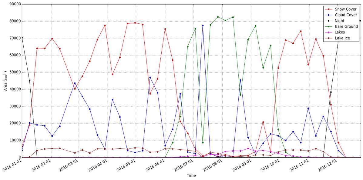
- Drawing the final graphs using the Plotting library (i.e., matplotlib.pyplot) to produce the final plots. The following three types of plots are provided by the code:
- “Area vs. Time” shown in Figure 1. This graph shows area in square kilometers for the following classes: Snow Cover, Cloud Cover, Night, Bare Ground, Lakes, Lake Ice.
- “Area as a percentage vs. Time” shown in Figure 2. This graph shows Snow area percentage and non-useful area percentage. Data for this graph is calculated as follows:
Non-useful area is calculated as a sum of the following classes: missing data, no decision, night, ocean, cloud, detector saturated, fill.
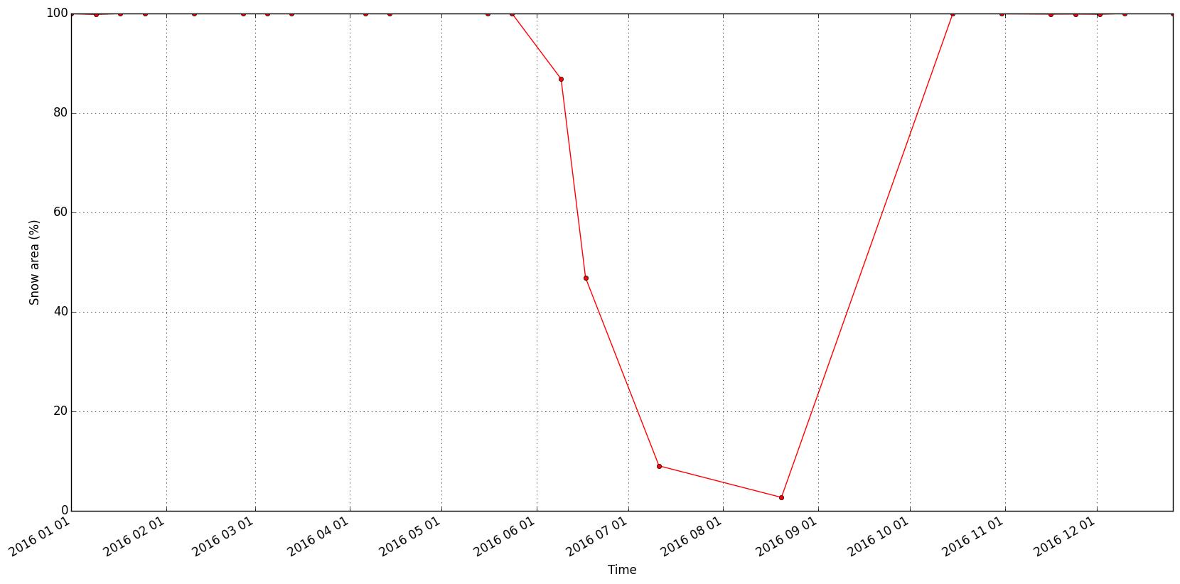
- “Snow area as a percentage vs. Time” shown in Figure 3. This plot shows snow data only for the periods when “Non-useful” area percentage does not exceed the threshold set by a user. Where the non-useful data exceeds the threshold, these points are excluded from the graph. This approach is based on an assumption that the percentage of snow cover area should be representative for the whole area unless the percentage of Non-useful area exceeds a threshold value provided by a user.
Table 1. MODIS data pixel values’ description (Hall & Riggs, 2016).
| Pixel Value/Class | Description |
| 0 | missing data |
| 1 | no decision |
| 11 | night |
| 25 | no snow |
| 37 | lake |
| 39 | ocean |
| 50 | cloud |
| 100 | lake ice |
| 200 | snow |
| 254 | detector saturated |
| 255 | fill |

References:
Esri. 2017. An overview of the Spatial Analyst toolbox. ArcGIS for Desktop. Retrieved from http://desktop.arcgis.com/en/arcmap/latest/tools/spatial-analyst-toolbox/an-overview-of-the-spatial-analyst-toolbox.htm
Hall, D. K. and G. A. Riggs. 2016. MODIS/Terra Snow Cover 8-Day L3 Global 500m Grid, Version 6. Boulder, Colorado USA. NASA National Snow and Ice Data Center Distributed Active Archive Center. doi: http://dx.doi.org/10.5067/MODIS/MOD10A2.006.