
Data Wrangling with Python and R, Part 2: LiDAR Validation with Differential GPS
One major part of my field season this past summer in the Yukon involved validating both of our LiDAR datasets with a differential GPS unit (dGPS for short). Independently quantifying survey accuracy is an essential part of any project involving LiDAR. Without knowing the LiDAR return accuracy in terms of elevation compared to the “true” ground surface, it’s impossible to tell how accurate any height-above-ground (HAG) metrics derived from the height-normalized point clouds might be.
LiDAR sensor manufacturers typically have listed accuracy values in their technical documentation, expressed in terms of 1-sigma (i.e., one standard deviation). According to documentation from their respective manufacturers, the Optech ALTM 3100 used for the 2007 survey has an accuracy of 15cm for surveys flying at 1200 m altitude above ground level, while the Riegl Q-780 used in 2018 is accurate to 2cm at a distance of 250m. However, independent validation campaigns are still needed as these tests are typically run under ideal survey conditions (i.e., low flight elevations, perfectly flat and hard surfaces) and may not apply for every given project.
In my field campaign, a Hemisphere S320 GNSS RTK system was used to collect several hundred dGPS points on relatively hard, flat surfaces such as roads and established ATV trails throughout the extent covered by both LiDAR surveys.
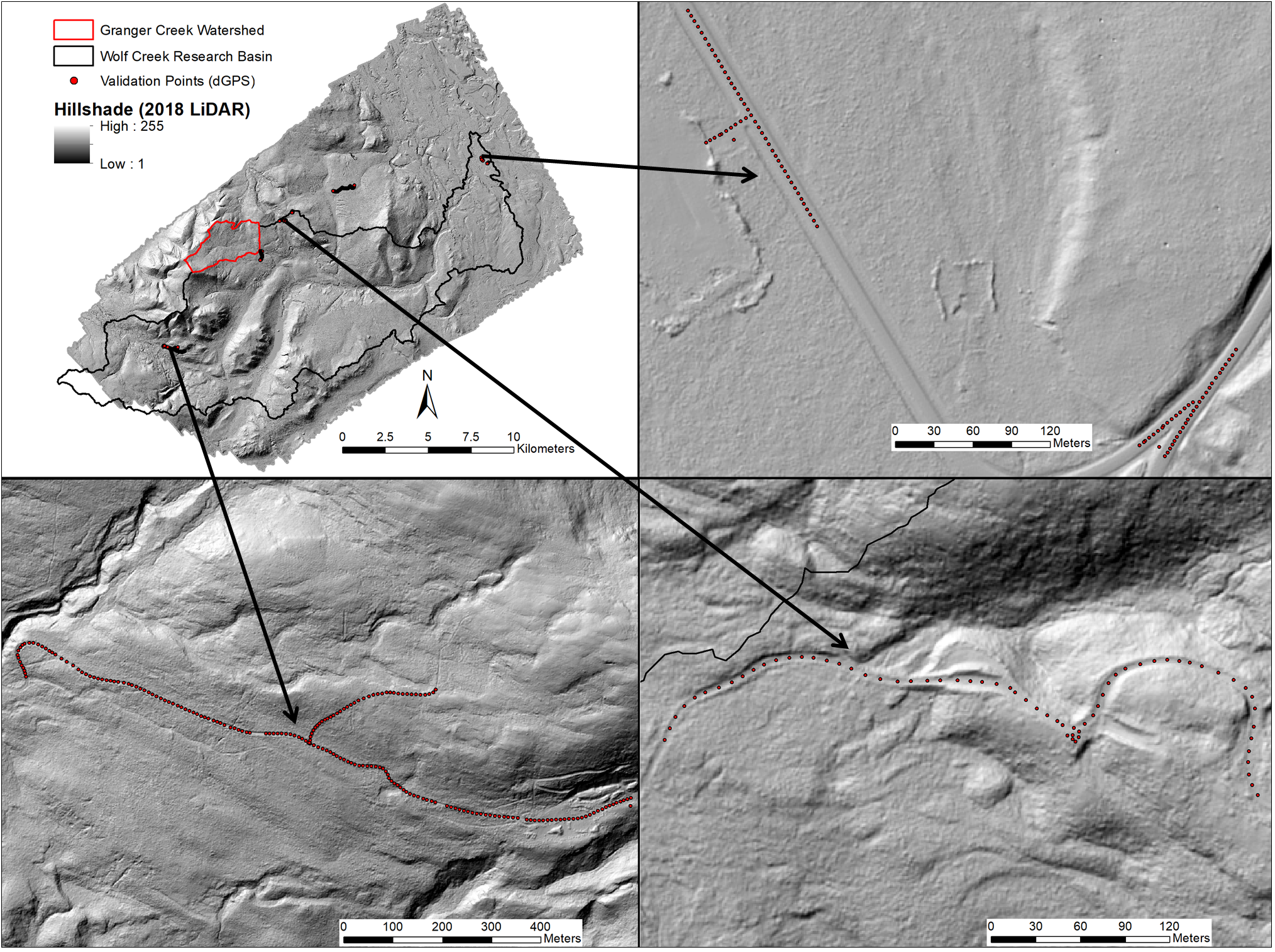
As this dGPS system was also used in the vegetation survey and shrubline mapping portions of the field campaign, any points from this vegetation work that captured an RTK Fixed position were included as a separate validation set to see how accurately the LiDAR could represent steeper, irregular terrain with substantial above-ground vegetation cover.

Before treating the dGPS coordinates as a true ground surface to compare our LiDAR to, they first needed to be post-processed to ensure they’re as accurate as possible. We configured our dGPS base station receiver in the field to record raw logging data every second it was transmitting for this purpose. These raw .BIN files include detailed information on the position and movement of GPS satellites referenced by the base station, atmospheric conditions throughout the survey period, and more.
Post-processing of the validation points was done using Natural Resources Canada’s Precise Point Positioning (CSRS-PPP) and TRX tools. CSRS-PPP uses precise GPS orbit and clock products generated through international collaboration to improve positioning results by a factor of 2 to 100 when compared to uncorrected positions. Once the dGPS raw logging files files are converted to RINEX format and run through CSRS-PPP, their “true” positions and shifts required to achieve them are provided in a detailed PDF over email.
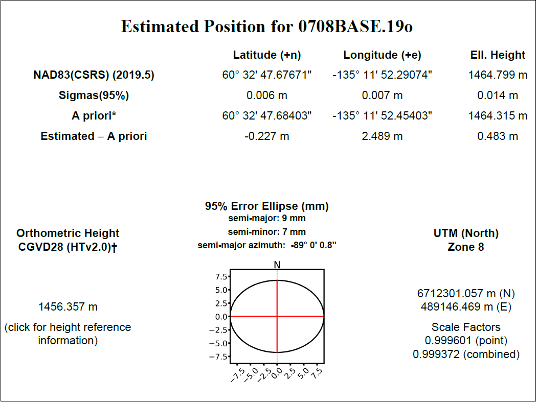
As CSRS-PPP computes estimated coordinates using the GRS80 ellipsoid, these averaged values had to be referenced to the WGS84 ellipsoid using the TRX tool so that they would match the 2018 LiDAR’s vertical and horizontal spatial references. The calculated shifts from these tools were then applied to the original dGPS output coordinates in CSV format and used to create new shapefiles in R. Here’s an example of how much a difference these corrections make when comparing our 2007 LiDAR elevations to the validation points using density plots:

We can see here that after post-processing with CSRS-PPP, the plot is much more well-distributed and the standard deviation of the residuals has decreased from 77cm to 14cm, which is just within the sensor manufacturer’s stated accuracy. This also applies for the 2018 point cloud comparisons, with standard deviations of 30cm and 7cm before and after applying the CSRS-PPP shifts.
As I’ll be comparing metrics from both LAS returns and LiDAR-derived rasters to my field data, we need to establish accuracy when comparing our dGPS points to both the original point cloud and interpolated DEMs. lascontrol is a tool that computes the height of a LiDAR point cloud at specified x and y control point locations by triangulating nearby points into a TIN, then reports the height difference relative to these control points. This was used to compare elevations from post-corrected dGPS validation points to last returns from the LiDAR and directly evaluate survey accuracy. After identifying and rasterizing last returns from the LAS tiles in LAStools and mosaicking the resulting GeoTIFFs together using the raster and rgdal packages in R, DEM elevations at validation point locations were extracted in order to compute height differences in ArcGIS.
Here’s how both LiDAR datasets compare to dGPS points from the vegetation surveys on much more complex terrain, in terms of both original LAS points and interpolated last-return DEMs:
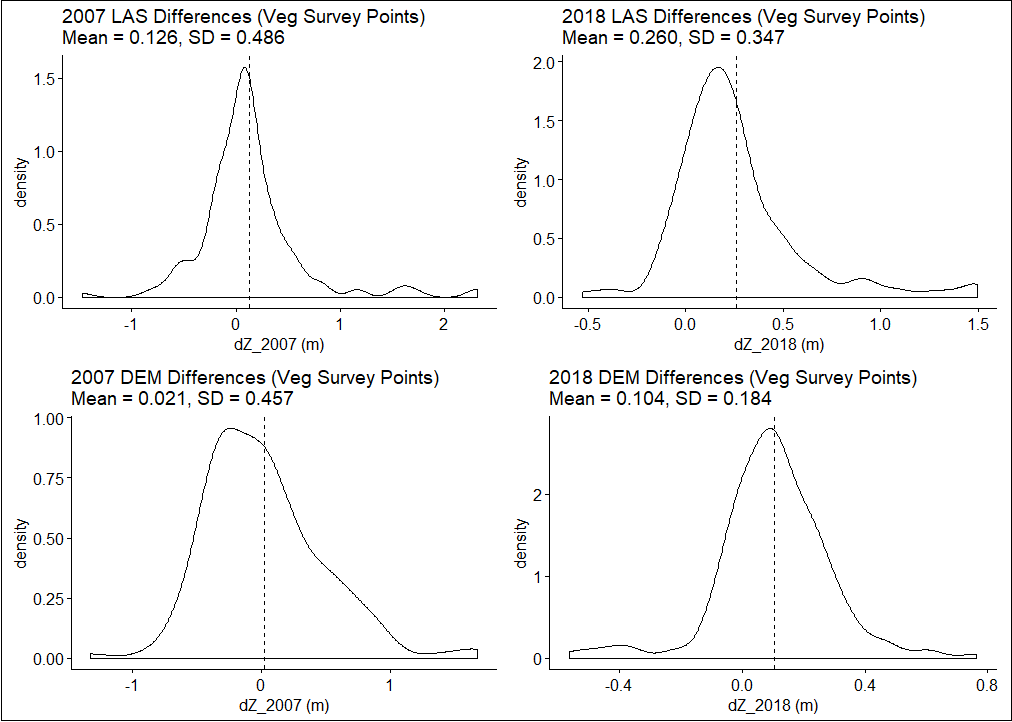
We can see now that when comparing dGPS points from the vegetation surveys to last-returns from the 2007 LiDAR dataset, the standard deviation (i.e., accuracy) of the residuals has jumped from a reasonable 14cm to over 48cm!
The results from this validation campaign show that while both surveys have around the same level of accuracy as reported by their respective sensor manufacturers on hard and flat surfaces, this gets much worse on more complex terrain (as expected). This is very important to know as I begin the next phase of my analysis, which involves directly comparing height-normalized LiDAR metrics at survey plot locations to their respective field-measured vegetation properties. Stay tuned!