
Modeling Line Features on DGGS Grids in the R-ArcGIS Environment
A Glance at DGGS
As a candidate for a new Earth reference standard, Discrete Global Grid System (DGGS) was confirmed by the Open Geospatial Consortium (OGC) as “a spatial reference system that uses a hierarchical tessellation of cells to partition and address the globe” in 2017. DGGS has been recognized as the most potential foundation of Digital Earth in the next generation. There are many keywords describing a DGGS: equal-area, tessellation, global domain, nested cells, unique index, to name just a few. Just try to imagine it as a hierarchical spreadsheet where cell locations are fixed at each resolution and spatial information can then be assigned to individual cells. A DGGS commonly begins with a Platonic Solid — an initial discretization of the Earth into planar cells, the initial cells are then be refined to an arbitrary resolution and mapped from planar cells to spherical cells by an equal-area projection method. OGC allows for a range of options to construct a DGGS, including different cell shapes, refinement ratio, projection methods, etc. For those who have not known much about it, I strongly suggest checking the References and Further Reading section; there is much to explore.
Model Line Features to Grids
Lately, I was working on a side project — uncertainties of geo-feature modeling on DGGS. The main goal for that project was to compare the geometric measurements and topological relationships among different configurations and granularities. To be clear here, DGGS grids are generated from inversely projecting planar cells to spherical cells instead of a simple tessellation process on a 2D plane. As one of the state-of-the-art DGGS implementations, the open-source R library dggridR provided all functions I need to generate DGGS grids within a certain region. However, to model a specific line feature (intersect grids with lines) and visualize the results seems to be more convenient in a professional GIS environment (e.g., ArcGIS). Thus, I think it would be good to work in both environment with an efficient bridge (e.g., the R library arcgisbinding). In this blog, I would like to show my way to model line features on DGGS cells in the context of ArcGIS Pro and R.
Vector data of major roads in Calgary, Canada were gained from the Open Calgary, the city of Calgary’s open data portal. In this blog, nine roads in the district 707G of Calgary were used as an example to show how the whole process worked. The roads have three types — Avenue, Street, and Trail, among which avenues are west-east directed, and the others are north-south directed. The original length for each road was calculated via geodesic distances (m). The length after conversion (m) was also calculated for the sample line features. In this experiment, the length after conversion was measured as the sum of straight-line-distances (geodesic) of cell centroids for the individual line feature.
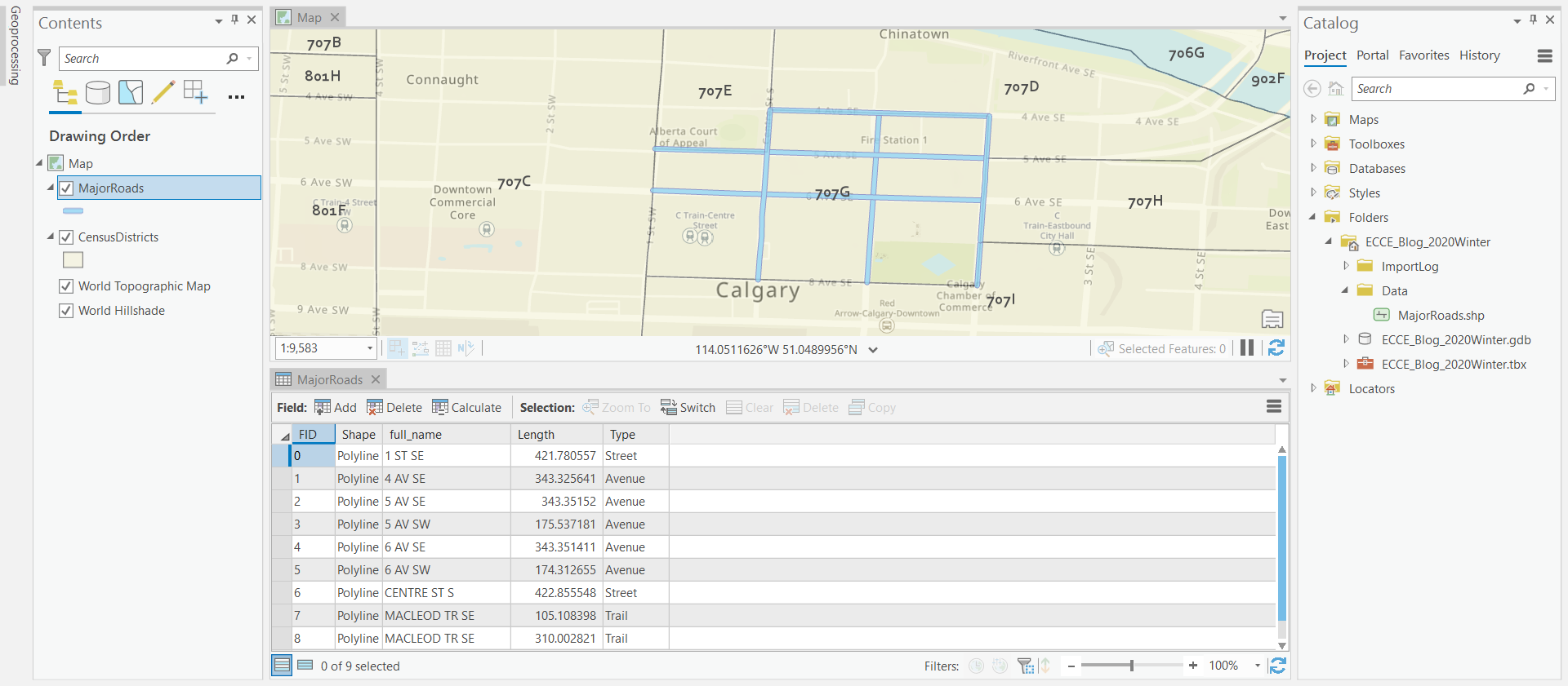
Figure 1. Nine target roads to be modeled in the district 707G, Calgary
Step 1. Generate DGGS grids with three different configurations covering the study area in the R environment
# Load libraries
library(dggridR)
library(rgdal)
library(ggplot2)

# Read the dataset
dsn.road = "H:\\UCalgary Courses\\ECCE_UC\\ECCE_Blog_2020Winter\\Data\\MajorRoads.shp"
MajorRoads = readOGR(dsn.road, layer="MajorRoads")

# Visualize the dataset
ggplot() +
  geom_polygon(data=MajorRoads, aes(x=long, y=lat, group=group), size = 1, fill=NA, color="black") +
  scale_y_continuous(name = "Longitude") + scale_x_continuous(name = "Latitude") +
  theme_classic() + coord_equal()

# Construct DGG objectS
dggs.ISEA4H.20 = dgconstruct(projection = "ISEA", aperture = 4, topology = "HEXAGON", res = 20, precision = 7)
dggs.ISEA4T.20 = dgconstruct(projection = "ISEA", aperture = 4, topology = "TRIANGLE", res = 20, precision = 7)
dggs.ISEA4D.20 = dgconstruct(projection = "ISEA", aperture = 4, topology = "DIAMOND", res = 20, precision = 7)

# Create DGGS grids and export as .shp files
dgshptogrid(dggs.ISEA4H.20, dsn.road, cellsize = 0.00001,
            savegrid = "H:\\UCalgary Courses\\ECCE_UC\\ECCE_Blog_2020Winter\\Data\\Roads_ISEA4H_20.shp")
dgshptogrid(dggs.ISEA4T.20, dsn.road, cellsize = 0.00001,
            savegrid = "H:\\UCalgary Courses\\ECCE_UC\\ECCE_Blog_2020Winter\\Data\\Roads_ISEA4T_20.shp")
dgshptogrid(dggs.ISEA4D.20, dsn.road, cellsize = 0.00001,
            savegrid = "H:\\UCalgary Courses\\ECCE_UC\\ECCE_Blog_2020Winter\\Data\\Roads_ISEA4D_20.shp")
Line 1-4: Load R packages needed for this step — dggridR; rgdal; ggplot2.
Line 6-8: Read the .shp file into the R environment as a Spatial Lines Data Frame.
Line 10-14: Visualize the target roads to be modeled in the R window (Figure 2).
Line 16-19: Define three grid configurations used in this experiment (ISEA4H, ISEA4T, and ISEA4D), all at the resolution level 20.
- ISEA4H — Icosahedral Snyder Equal Area Aperture 4 Hexagonal Grid (cell spacing = 6.7 m at resolution level 20)
- ISEA4T — Icosahedral Snyder Equal Area Aperture 4 Triangular Grid (cell spacing = 3.9 m at resolution level 20)
- ISEA4D — Icosahedral Snyder Equal Area Aperture 4 Diamond Grid (cell spacing = 6.7 m at resolution level 20)
Line 21-27: Create grid cells with different configurations in the study area and save them as .shp files.
Figure 3 visualizes a section of generated hexagonal grids in the ArcGIS Pro environment.
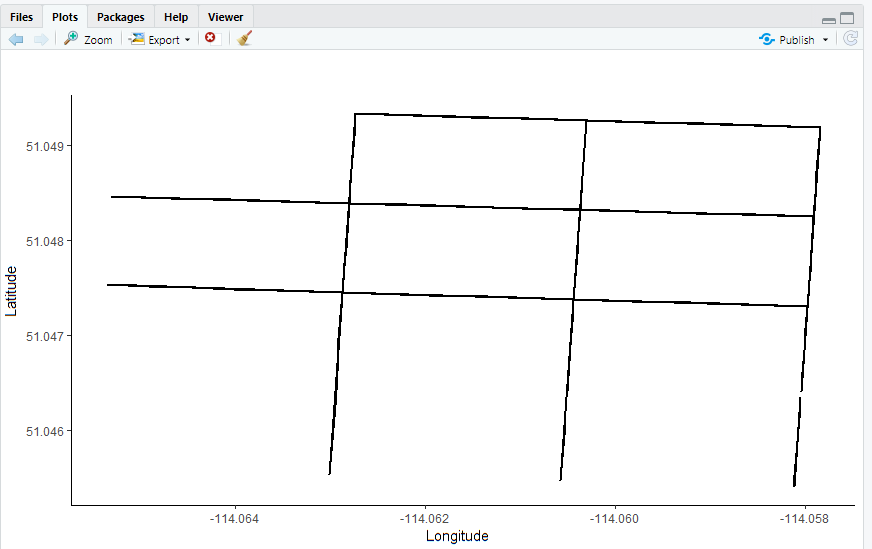
Figure 2. Visualization of the raw roads in R

Figure 3. Visualization of a section of the hexagonal grids in ArcGIS Pro
Step 2. Detect grid cells representing individual roads in the ArcGIS Pro environment
## Set the working envrionment
env = r"H:\UCalgary Courses\ECCE_UC\ECCE_Blog_2020Winter\ECCE_Blog_2020Winter.gdb"
arcpy.env.workspace = env
arcpy.env.overwriteOutput = True

InputFeature  = "Roads_ISEA4H_20" # Roads_ISEA4T_20 / Roads_ISEA4D_20
SpatilJoinOutput = "Roads_ISEA4H_spjoin" # Roads_ISEA4T_spjoin / Roads_ISEA4D_spjoin

## Spatial join the grid shapefile and the road shapefile
arcpy.SpatialJoin_analysis(InputFeature, "MajorRoads", SpatilJoinOutput, "JOIN_ONE_TO_MANY", "KEEP_COMMON", '', "INTERSECT", None, '')

## Add fields to store latitude and longitude values
arcpy.AddField_management(SpatilJoinOutput, "longitude", "DOUBLE")
arcpy.AddField_management(SpatilJoinOutput, "latitude", "DOUBLE")

## Calculate latitude and longitude for the cell centroids
arcpy.management.CalculateGeometryAttributes(SpatilJoinOutput, "longitude CENTROID_X;latitude CENTROID_Y", '', '')
First, spatial join the generated grids with the MajorRoads shapefile, with the JOIN ONE TO MANY option and only keep those records with INTERSECT relationships. Then, calculate the lat/lon coordinates of cells centroids. Repeat the same operation for three datasets of different grid types. This step can be done manually with ArcGIS tools, while the above shows the Python script accomplishing the same task. Figure 4-6 visualize the road representation by hexagonal, triangular, and diamond cells, respectively.
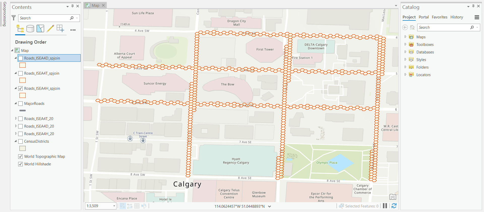
Figure 4. Represent roads by hexagonal cells

Figure 5. Represent roads by triangular cells
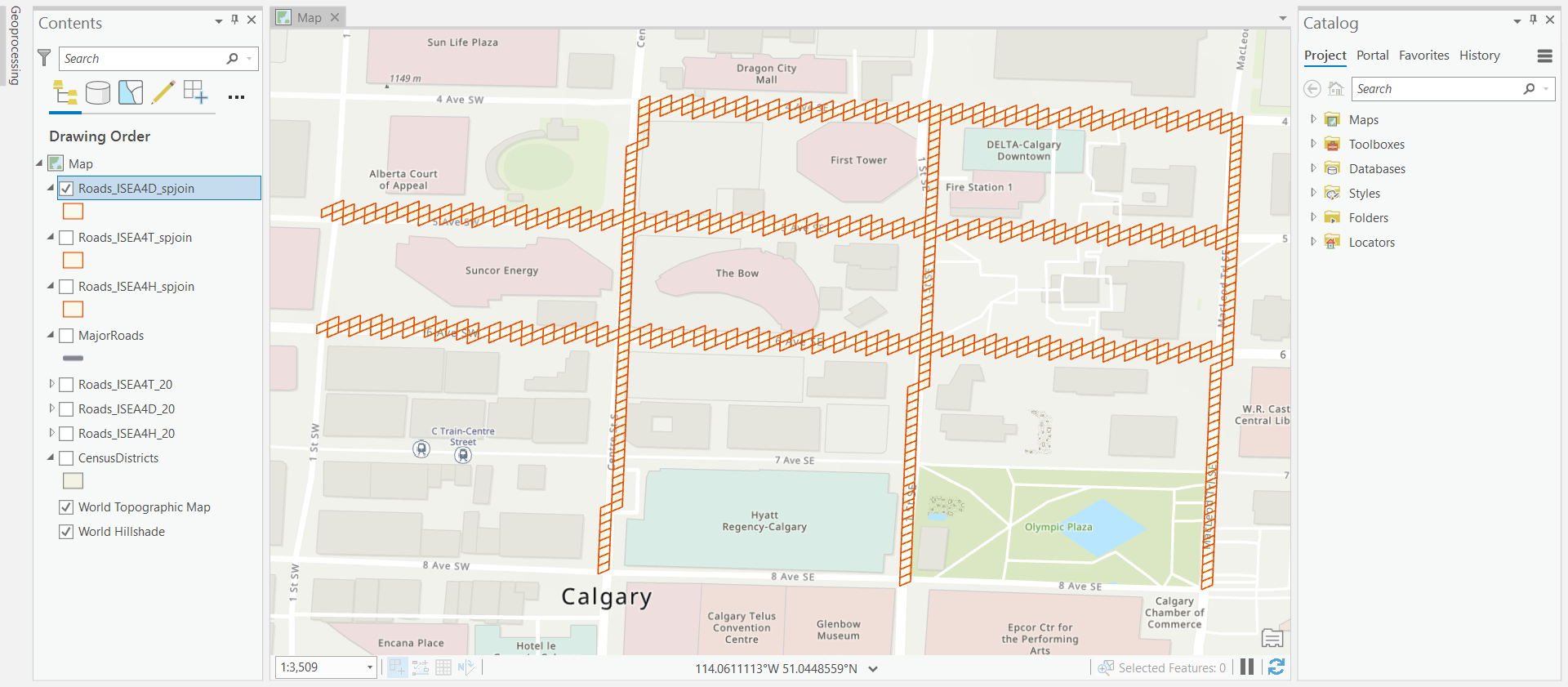
Figure 6. Represent roads by diamond cells
Step 3. Calculate the new road length after conversion in the R environment
# Load libraries
library(arcgisbinding)
library(dplyr)
library(geosphere)

# Print information regarding the ArcGIS product and license
arc.check_product()

# Open the datasets
Rd.ISEA4H = arc.open("H:/UCalgary Courses/ECCE_UC/ECCE_Blog_2020Winter/ECCE_Blog_2020Winter.gdb/Roads_ISEA4H_spjoin")
Rd.ISEA4T = arc.open("H:/UCalgary Courses/ECCE_UC/ECCE_Blog_2020Winter/ECCE_Blog_2020Winter.gdb/Roads_ISEA4T_spjoin")
Rd.ISEA4D = arc.open("H:/UCalgary Courses/ECCE_UC/ECCE_Blog_2020Winter/ECCE_Blog_2020Winter.gdb/Roads_ISEA4D_spjoin")

# Create a new dataframe to store results
ISEA4H.df = ISEA4T.df = ISEA4D.df = data.frame(StreetID = integer(), ConvertLength = double())
# create a vector to store street ID
road.id = (0:8)

# Creat a function to calculate the road length after being converted on DGGS grids
# Two parameters included road ID and the input dataset with different grid types
polyline.length = function(roadid,inputdf){
  # Import the subsection of the attribute tables
  df = arc.select(object = inputdf, fields = c('JOIN_FID','Type','longitude','latitude'))
  # Select those cells corresponding to a specific road
  road.matrix = filter(df, (JOIN_FID == roadid))
  # If the road is west-east directed (type is Avenue) then sort cells by longitude firstly
  # If the road is north-south directed (type is not Avenue) then sort cells by latitude firstly
  if(road.matrix$Type[1] == "Avenue"){
    centroid.matrix = road.matrix[,c("longitude","latitude")][order(road.matrix$longitude, road.matrix$latitude),]
  } else {
    centroid.matrix = road.matrix[,c("longitude","latitude")][order(road.matrix$latitude, road.matrix$longitude),]
  }
  # Calculate the the length after conversion
  Convert.length = lengthLine(centroid.matrix)
  # Report the converted length
  results = c(roadid,Convert.length)
  return(results)
}

# Call the function in three loops
for (rid in road.id) {ISEA4H.df = rbind(ISEA4H.df, polyline.length(rid,Rd.ISEA4H))}
for (rid in road.id) {ISEA4T.df = rbind(ISEA4T.df, polyline.length(rid,Rd.ISEA4T))}
for (rid in road.id) {ISEA4D.df = rbind(ISEA4D.df, polyline.length(rid,Rd.ISEA4D))}

# Summary all info in a new data frame for comparison
ConvertSummary = data.frame(MajorRoads)
ConvertSummary$ISEA4HLength = ISEA4H.df[,2]
ConvertSummary$ISEA4TLength = ISEA4T.df[,2]
ConvertSummary$ISEA4DLength = ISEA4D.df[,2]
Line 1-4: Load the packages needed — arcgisbinding; dplyr; geosphere.
Line 6-7: Print information regarding the ArcGIS product and license on this machine.
Line 9-12: Import the datasets of the grid cells representing individual roads.
Line 14-15: Create new data frames to store the calculation results.
Line 16-17: Create a vector to store road ID from 0 to 8.
Line 19-38: Create a function to calculate the new road length. The length was calculated as the sum of straight-line-distances (geodesic) of cell centroids for each road. Before calculation, the cell records needed sorting by their spatial locations. If the road is west-east directed, sort the cells by ascending longitude then ascending latitude; if the road is north-south directed, sort the cells by ascending latitude then ascending longitude.
Line 40-43: Call the newly created function for each road with each grid configuration.
Line 45-49: Summary all the converted length on various grid configurations for comparison. The comparison results are in Figure 7.
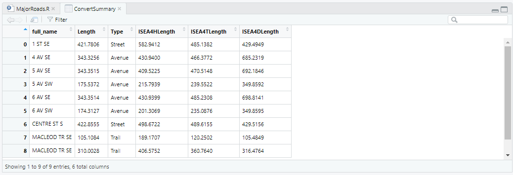
Figure 7. Comparison of the new length on various grid configurations with the original road length
The converted length was always greater than the original ones, that was because of the jagged, rasterization-like representation on the DGGS grids. This was a simple example showing the modeling process at a coarse resolution for a clear illustration. As the resolution of the grid increases, the length measurement accuracy will be much improved.
I hope this blog provides some insight into working with R-ArcGIS environment and how to use a DGGS.
References and Further Reading
- Discrete Global Grid Systems – A New OGC Standard Emerges
- Bring It All Down to Earth with DGGS
- Geodesic Discrete Global Grid Systems
- A Survey of Digital Earth
- Digital Earth Platforms
- Next-generation Digital Earth
- Discrete Global Grids: A Web Book
- A New Standard from the OGC Promises to Right One of Spatial’s Longest Standing Problem: its dependence on latitude and longitude