
The Importance of Scale (A brief introduction)
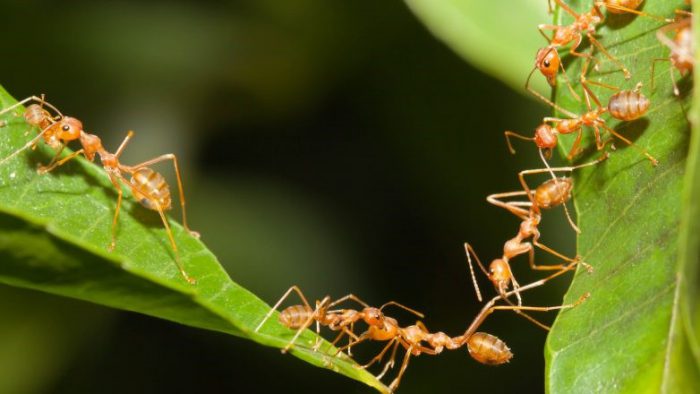
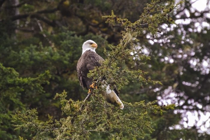
When we look at life from the viewpoint of an ant, and then compare it to that of a soaring bald eagle, we come to the realization that they are quite markedly different from one another. What may seem like a mountain for an ant to climb is just a rock settling in between the talons of an accipiter. If we make time negligible, the entire life of an ant might be spent within a 0.5km2 radius, while that of a bald eagle can extrapolate to 5km2 (area is in reference to the average home range). Similarly, a single rain drop can act as a defiant force of gravity to an ant, however, it is a mere speck of water that will seamlessly slide off the eagle’s scapular feathers. All this is to say that the way in which we view the interactions individuals have with their surrounding environments differ between species, between populations, and between ecosystems. They differ from local levels as compared to regional levels, and even extending to global levels. What does this all come down to? Why is the life of an ant or eagle important to consider? How does this have anything to do with GIS you ask? Scale. A critically important word when it comes to studying ecological interactions, especially interactions that incorporate a spatial component.
In a recent book published by Worm and Tittensor (2018), the authors highlight the importance of critical thinking when dealing across multiple spatial and temporal scales. In this context, the concept of spatial scale is in reference to the geographical extent of study of species (e.g., large global vs. small local populations). For example, at varying spatial scales, species richness will correlate with different predictors (Worm & Tittensor, 2018). What they found was that net primary productivity is a dominant predictor for species richness at smaller scales, while temperature has the largest influence at larger scales (>1000km) (Worm & Tittensor, 2018). In essence, the scale at which you deal with your data depends on the question you are asking. At local scales, diversity is more likely to be shaped by species interactions, environmental constraints, and even human impacts on the local habitat (Worm & Tittensor, 2018). However, if the primary concern is attempting to understand the size and distribution of species pools in the first place, the scale must be larger and have a more coarse representation. This is because the variables that are dominant at local scales have less of an effect on distribution patterns as we zoom out and include larger areas of study.
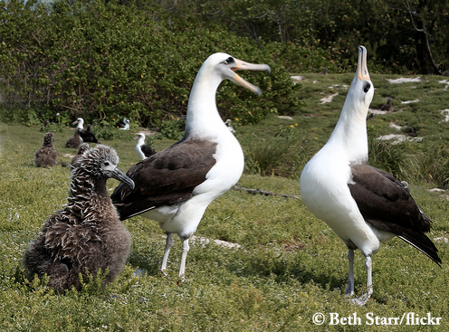
Now think closely, if we were to study a population of say, albatross on the Galapagos Islands, what may influence the diversity and/or success of these species may have to do with intra- and interspecific competition, resource availability, or primary productivity. However, if we were to study the global diversity of all albatrosses – including ranges in Antarctica, Australia, New Zealand, South Africa, South America, the North Pacific, and the Galapagos Islands – their influences might be more highly correlated to temperature and seasonality. What affects a Family at one scale can change as you extrapolate outwards and begin to incorporate larger areas and more species.
GIS can help us put all the abiotic variables onto the same scale, allowing us to interpret and analyze our questions accordingly. The tricky part here is determining which scale is the most appropriate for the questions you are asking. If your scale is too small, you might create too much “noise” in the data, making it difficult to identify and interpret any trends. However, if the scale is too large, you risk generalizing the data too much, and blurring any notations of a change in the patterns of your data. Typically, the appropriate scale is found by: (1) considering the questions you are asking, (2) performing a thorough literature review on other papers who have also analyzed data at a similar level, and (3) at times, trial and error in exploring the patterns your data show at varying spatial scales.
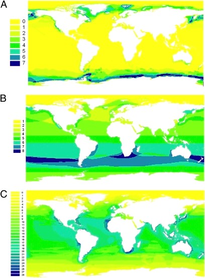
I have found this “realization” and understanding of the importance of scale to be particularly applicable to the research I am working on. I am attempting to understand the abiotic correlates that are driving global diversity patterns of Chondrichthyans (sharks, rays and chimeras), and how we can use those abiotic predictors to aid in current and future conservation prioritization. As an example, look at the figure below and ask yourself how it might differ if we were to change our spatial scale from a global analysis to understanding species richness patterns strictly along the eastern coast of Australia. There is always a lot to think about and consider when dealing with species distributions and how that can enlighten our path to improved conservation methods.
Until next time! When I have hopefully developed further into my masters! 🙂
Pompa, S., Ehrlich, P.R., and Ceballos, G. 2011. Global Distribution and Conservation of Marine Mammals. Proc Natl Acad Sci USA 108(33): 13600-13605
Worm, B., and Tittensor, D.P. 2018. A Theory of Global Biodiversity. Princeton, NJ: Princeton University Press.