ECCE App Challenge 2018 – Marauders mApp
This year I participated in the ECCE App Challenge with my group members, Tasos Dardas and Matt Brown. The assigned topic of the app was anything of our choice, so we decided to focus on decentralized, renewable energy. Our app, Energy Revolution, demonstrates the feasibility of decentralized energy systems (DESs) by creating matrices showing the potential, renewable energy that can be generated from each dissemination area (DA) in Calgary. This app considers two sources of renewable energy, solar and biogas. Part of my role in the development of the app was to quantify the solar potential of each building in Calgary.
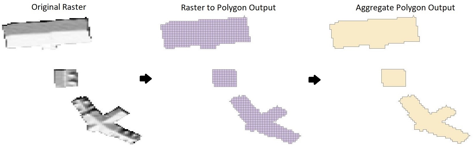
From the Calgary open data catalogue, I found a raster dataset created by the city that quantifies the potential solar energy of all buildings within the city. The processing of the data took many hours in order for the information to be utilized in our app. First, the data was converted from a raster to polygons in order for the user to click on each individual building. The high resolution of the solar data showed a single building with differing values of solar potential energy, causing a single building to be made up of multiple polygons. For the purpose of this app, we wanted to quantify the average amount of solar energy for each building. To do this, I used the Aggregate Polygons tool in ArcMap by inputting the polygon layer and specifying an Aggregation Distance of 1 meter. I assumed buildings are at least 1 meter apart so any polygons within 1 meter of each other were combined into a single polygon. However, the attributes of the polygons were not retained as the result did not have the solar potential of each building. By employing a Spatial Join between the layer with multiple polygons for a single building and the layer with a single polygon for each building, I summarized the solar potential of each building by assigning the sum to the single polygon building layer.
There was a total of 16 rasters in the solar potential data created by the city, with many of the files being over 300 mb. The high resolution, 1.42 meters by 0.89 meters, made processing of a single tool take hours at times. Due to the limited time, the fastest was to convert the data was to use multiple computers in the GIS lab to process a single raster on each computer. Overall, the task was completed in about 9 hours.